Communicating between the computer and a circuit board (sending and receiving voltages from the computer) is accomplished with the data acquisition card (DAQ). The DAQ is normally connected from the computer to the circuit board with a 68-pin cable. In general, all 68 pins are used for such things as analog inputs and outputs, triggering, digital inputs and outputs, a 5-V dc supply, and counters. In our projects, we use, for the most part, only analog inputs and outputs. A digital output could also be used if we required an additional output, which of course is limited to on or off.
Since the
analog inputs and outputs involve digital-to-analog and analog-to-digital
conversions, special consideration must be given to the discrete nature of the
conversion relations. These are discussed in the following along with a series
of basic programming and measurement exercises. A sequence of
The LabVIEW
library, ProjectA.llb, of Project
A
contains the preprogrammed VIs, along with samples of all of the
|
Project PA.x (Title of Project Segment) |
![]()
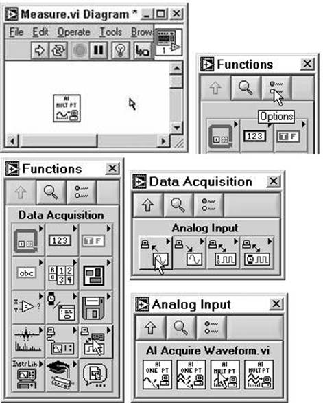
A.1 Basics of Sending and Receiving Circuit VoltagesThe following is based on a National Instruments PCI-MIO-16E-4 DAQ card (or equivalent). The sample rate is not critical. The DAQ card has eight differential analog input channels and two analog output channels. We generally use only channels 0, 1, and 2 for receiving in our projects. LabVIEW
provides some preprogrammed As the name suggests, the VI, AI Acquire Waveform.vi samples the stipulated voltage a number of specified times. For dc measurements, the samples are simply averaged. This provides for a more precision measurement than from a single sample. LabVIEW has a single-point DAQ function, AI Sample Channel.vi. This function does not take advantage of computer-based data acquisition. A.1.1 Programming
Exercise: Installing, Sending, and Receiving
|
||||||||||||
|
TABLE A.1 |
||
|
Diagram |
Tools Palette Functions Palette Or Menu Sequence: |
Shift/Right Click Right Click - Stickpin to hold Window>>Show Functions Palette |
|
Front Panel |
Tools Palette Controls Palette Or Menu Sequence: |
Shift/Right Click Right Click - Stickpin to hold Window>>Show Controls Palette |
When installed, AI Acquire Waveform.vi appears as in Fig. A.1. Now Double Click on the icon (or Right Click and Open Front Panel) to bring up the Front Panel of AI Acquire Waveform.vi. It will appear similar to the example shown in Fig. A.2, which has some cosmetic changes.
The Digital Controls in the Front Panel of AI Acquire Waveform.vi provide for installing the machine device number (e.g., 1), the input channel, number of samples, and sample rate in addition to the ADC (analog-to-digital converter) Digital Controls high limit and low limit. The default, 0 V, as in the example, is equivalent to 10 V and -10 V for high limit and low limit, respectively.
The device number of the DAQ card is set using the National Instruments Measurement & Automation utility. Go to Start>>Programs>>National Instruments>>Measurement & Automation. This opens a window called Max. Then under My System, locate Devices and Interfaces and Right Click on the name of the DAQ card to bring up Properties. The device number can be set from the Properties window. The sample programs in ProjectA.llb use Device 4 (or as set on your PC). Close Max.
We will want to send out some voltages to be read by the input channel. For this, add output channel function AO Update Channel.vi to the Diagram of your VI. It is under Functions>>Data Acquisition>>Analog Output. Install this VI in your VI diagram as shown in Fig. A.3. Position the icons with the Positioning Tool (arrow). It is obtained by cycling through the Tools by striking the Tab key or Space Bar, or, again, get the Tools Palette with Shift/Right Click from the Front Panel or Diagram.
|
Project PA.1 Sending and Receiving Voltages with the Sending and Receiving VIs (Measure.vi, version 1) |
The two
For ensuring proper execution order, install a Sequence Structure as shown in Fig. A.4. Obtain the Sequence Structure from the Diagram under the menu series Functions>>Structures>>Sequence. Recall that to obtain the Functions Palette, Right Click on the Diagram.
Initially, the Sequence Structure is too small. To enlarge, get the Positioning Tool (arrow) by pressing the Space Bar, by sequencing through the Tools with Tab, or by using Shift/Right Click to bring up the Tools Palette. Position the Tool at the lower-right-hand corner of the Sequence Structure, Left Click, and drag to enlarge the Structure.
Right Click on the edge of the Frame of the Sequence Structure and go to Add
Frame After (Fig. A.4). The result will be two Frames with index 0 and index 1. Now place
(e.g., drag) the send and receive
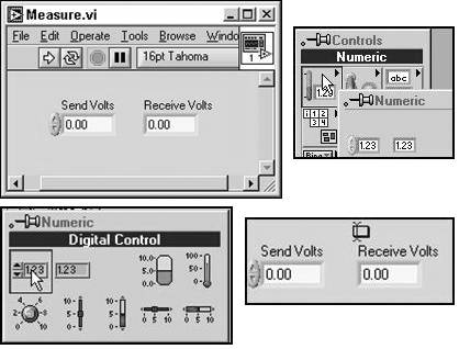
The Front Panel of Measure.vi will now be configured to permit assigning the voltage to be sent out and reading the input voltage from the Front Panel. The Front Panel of the new configuration is shown in Fig. A.5. From the Front Panel and then from the Controls Palette, go to Controls>>Numeric (Fig. A.5), and from this selection, get a Digital Control and a Digital Indicator. You might want to color the Front Panel. For this, Shift/Right Click and get the Coloring Tool from the bottom of the Palette. Then, with the Coloring Tool, Right Click on the Front Panel and pick a color. You can also color the Diagram. Change the labels over the Digital Control and Digital Indicator using the Edit Text Tool (Fig. A.5). Obtain the Tools Palette with Shift/Right Click and the Edit Text Tool. The labels are defaulted as Numeric. Use the Edit Text Tool from the Tools Palette to relabel as in the example (or similar).
Now go to the Diagram (under Menu Window>>Show Diagram or use Ctrl E) for wiring the program in the diagram. This will include Terminals and Numerics and Strings. Start by connecting the sending VI icon (Frame 0) value to the Digital Control terminal (Fig. A.6). To locate the terminal for the Digital Control, go back to the Front Panel, Right Click the Digital Control for Send Volts, and move the pointer to Find Terminal. The Diagram will open and the proper terminal will be highlighted. Note that the terminal for Digital Control is darker than those for Digital Indicator. This provides for an alternative means of locating the proper terminal.
Get the Wiring Tool (appears like a roll of solder) by striking the Space Bar. To wire, first find the correct terminal on the icon. There are three in this case. The terminal for this connection, value, is the bottom third of the icon. To locate the region of the connection, sweep the Wiring Tool over the icon and find the value. A given terminal displays a black-and-white blinking while the Wiring Tool is in contact with this terminal. Now, with the Wiring Tool, Left Click on the value connection region, Release, and move the Wiring Tool to the terminal of the Digital Control. Left Click again to finish.
For an alternative view of where the connections are made, you can Right Click on the icon, and get Visible Items>>Terminals. Recall again that the Digital Control terminal is darker than the Digital Indicator terminal. This adds additional clarification as to the correct terminal.
Complete the connections to the icon with a Numeric Constant for the device (Right Click, then Functions>>Numeric>>Numeric Constant) and a String Constant for the channel (Right Click, then Functions>>String>>String Constant). Use the Pointing Tool (finger) to write in the constant values. Obtain the various Tools by striking the Tab key.
Now sequence to Frame 1 to connect to the AI Acquire Waveform.vi icon. (Click on the arrows at the top of the Sequence Structure.) Complete all wiring, as shown in Fig. A.6, except for the waveform terminal (connection on the right side of the icon in Frame 1). This includes device (numeric constant, 4), channel (string constant, 0), number of samples (numeric constant, 100), high limit (numeric constant, 10), and low limit (numeric constant, 0). The low limit can be set to 0 because no negative numbers are to be read.
As a reminder for using the Wiring Tool: In the Diagram, use Shift/Right Click to get the Tools Palette and obtain the Wiring Tool. The Wiring Tool is also obtainable by pressing the Space Bar, while the Diagram is the active window, to sequence between the Wiring Tool and the Positioning Tool. Left Click on the terminal to be wired (do not hold) and move the Tool to the other termination and Left Click again.
To complete connections to the terminals associated with Frame 1, we must add the VI Mean.vi (Fig. A.7). It is used to obtain the average of all of the number of samples (as selected) in the reading (receiving) function. Note that Mean.vi is connected between the waveform terminal of the AI Acquire Waveform.vi and the Digital Indicator terminal. The output from AI Acquire Waveform.vi (waveform) in this case is a cluster of information including a data array. In the Diagram, a much broader line than that for a single data point represents the connection.
Mean.vi is obtainable from two different locations in the Functions palette: Functions>>Analyze>>Mathematics>>Probability and Statistics>>Mean.vi;Functions>>Mathematics>>Probability and Statistics>> Mean.vi. Connect the waveform of the Frame 1 icon to Mean.vi to the Digital Indicator Terminal. Connect the output in Mean.vi, mean, to the Terminal of the Digital Indicator. This measurement, which is the average of a large number of samples, is superior to obtaining a single point that might very well fluctuate due to noise.
|
Project PA.2 Sending and Receiving Voltages from the Front Panel (Measure.vi, version 2) |
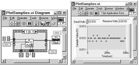
A given dc voltage is sent out via an output channel (e.g., frame 0 of Fig. A.7). A circuit node response is measured, in our projects, by sampling the voltage a number of times. With LabVIEW, we can easily obtain a graphical presentation of the sample data points to provide an indication of the noise that exists on the dc voltage being measured and in the measurement system. For this, obtain a new VI by saving a Save As copy and giving it a new name. Here it is named PlotSamples.vi. The new VI will initially appear something like that in Fig. A.8
To install the Waveform graph, in the Front Panel, Right Click and get Controls>>Graphs>>Waveform Graph and place it on the Front Panel. Shift/Right Click on the face of the graph to get the Coloring Tool and pick a color for your graph background field and Frame. Figure A.8 shows a new graph installation with some color changes.
A new installation of a graph has the Plot Legend open (Plot 0 in the example). In general, this feature and others can be hidden or made to appear by a Right Click anywhere on the graph and then selecting Visible Items as shown in the example of Fig. A.9
In the box of the Plot Legend, Right Click, go to Color and pick a color for the plotting points or lines. Also, select Points under Common Plots. Hiding the Plot Legend might be in order, now although this is optional. (Right Click on the graph face and select Visible Items>>Plot Legend.)
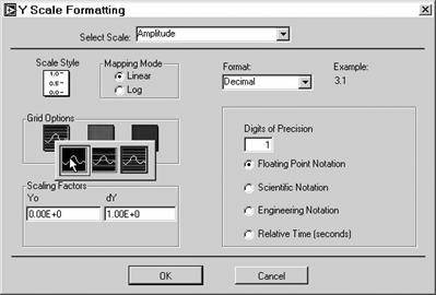
For the present application, it is preferred to have no grid. To accomplish this, Right Click on a number on the Y-scale of the Frame of the graph, go to Formatting... and Grid Options (Fig. A.10). Select the no grid (Left Click) condition as illustrated in Fig. A.10. Repeat for the X-axis. Note that a given axis can be selected from the Formatting window at the top under Select Scale.
Now use the Edit Text Tool to edit the X and Y designators. Then Right Click on the graph face and get Find Terminal. Complete the wiring to the graph terminal as in Fig. A.11. The final Front Panel (Fig. A.11) has the label hidden and the X- and Y-axis designators edited to be Sample Value(V) and Time (sec). The graph data are from a sample measurement from Project A
|
Project PA.3 Plotting Measured Samples (PlotSamples.vi) |
Very often in measuring circuit characteristics, it is necessary to plot some voltage response over a wide range of input-voltage stimulation. An automatic means of adjusting the voltmeter sensitivity through the sweep is thus required. When set for the full measurement range (limit), the 12-bit analog-to-digital conversion (ADC) in the DAQ has either a 2.44 mV (unipolar, 10 V full range) or a 4.88 mV (bipolar, 20 V full range) resolution.
However, the range of the DAQ is software selectable. So, for example, suppose that in the sweep we are measuring 5 mV and only positive voltages. The DAQ can be programmed for a high limit of, for example, 100 mV and a low limit of 0 V (unipolar), such that the resolution is 24.4 mV.
The Project A LabVIEW library, ProjectA.llb, contains a preprogrammed VI for setting automatically the range. The Diagram of the VI, Voltmeter.vi, is shown in Fig. A.12. As indicated, the range is set through the high- and low-limit inputs to AI Acquire Waveform.vi, for example, 10 V (high limit) and 0 V (low limit) in the diagram of our autoranging voltmeter as shown in Fig. A.12
The autoranging voltmeter is programmed as follows. First, a copy of AI Acquire Waveform.vi is Saved As..., modified for dc only and renamed as AI Acquire Avg.vi. The modification consists of taking the average of the array of samples and providing for a single-point output of the average value of the samples. AI Acquire Avg.vi is programmed to operate in selectable bipolar or unipolar mode. Thus, this feature is included in Voltmeter.vi.
This VI is
then used as a subVI in the autoranging dc voltmeter. Upon running Voltmeter.vi, the execution starts with the subVI AI Acquire Avg.vi on the left; the high limit set at
10 V, and with the bipolar mode, the lower limit is -10 V. Thus the voltage
being measured is first sampled with minimum sensitivity but this is sufficient
to obtain an approximate value of the voltage. The initial measurement value is
then processed through a selection scheme to decide which limit should be set
into the final measurement subVI that is again AI
Acquire Avg.vi. The limit choices are given in Table
A.2.
These are stored in an Array Digital Control as seen on the left in the diagram![]() . The While Loop compares the
measured value with each limit value starting at the top. The loop halts when
the comparison finds the smallest possible limit. Bipolar or unipolar are set
according to the sign of the initially measured value.
. The While Loop compares the
measured value with each limit value starting at the top. The loop halts when
the comparison finds the smallest possible limit. Bipolar or unipolar are set
according to the sign of the initially measured value.
A factor of 2 of improved resolution is available with the unipolar case. As noted, the valid limit settings and associated resolutions are shown in Table A.1. With the autoranging voltmeter, during a sweep, the resolution is maintained, through the sweep, at roughly a fixed percentage of the value of the numbers being measured.
|
TABLE A.2 |
|||||
|
Unipolar |
Range |
Resolution |
Bipolar |
Range |
Resolution |
|
0 to +10 V |
2.44 mV |
-10 to +10 V |
4.88 mV |
||
|
0 to +5 V |
1.22 mV |
-5 to +5 V |
2.44 mV |
||
|
0 to +2 V |
mV |
-2 to +2 V |
1.22 mV |
||
|
0 to +1 V |
mV |
-1 to +1 V |
mV |
||
|
0 to +500 mV |
mV |
-500 to +500 mV |
mV |
||
|
0 to +200 mV |
mV |
-200 to +200 mV |
mV |
||
|
0 to +100 mV |
mV |
-100 to +100 mV |
mV |
||
|
-50 to +50 mV |
mV |
||||
Figure A.13 shows a measurement of a sine-wave from a function generator. This was obtained in LabVIEW using the ac voltmeter that is discussed in a following unit. The voltage waveform is sampled at the two limit settings, 100 mV (a) and 2 V (b). The peak of the sine-wave is 10 mV. It is clear that the resolution is not adequate at the higher limit setting. In an autoranging version of the ac voltmeter, the best limit setting is automatically assigned.
|
Project PA.4 Using the Autoranging Voltmeter |
An example of an oscilloscope is shown in Fig. A.14. This special version displays three waveforms. These are the total waveform (ac + D), the sine-wave minus the dc (average value) and the absolute value of the sine-wave (|ac|).
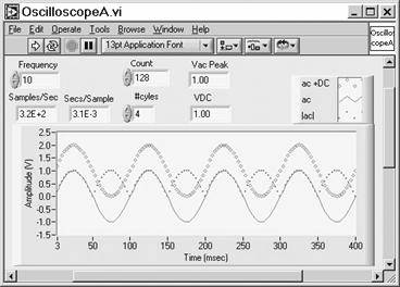
The voltmeter is designed to measure peak or RMS values for periodic waveforms, thus, to be an ac voltmeter. Total sampling time must occur in exact multiples of cycles. This provides for obtaining the waveform (sine-wave) peak or RMS value based on an average of all the samples.
The required sample rate, SR, is obtained from
![]()
The values for all the numbers on the right-hand side are set in Digital Controls on the Front Panel (Fig. A.14). The #Samples is also referred to as the Count.
SR and #Samples are then sent to the subVI, AI Acquire Waveform.vi. For example, assume that the #Cycles is 4 and the #Samples is 256. Once cycle will be sampled 64 times. Assume also that f = 1000 Hz. Sample rate SR will be 64000 samples/sec or about 16 msec/sample. The total sampling time is T · #Cycles, where T is the period and is T = 1/f. In this example this is 4msec.
Digital
Indicators in the Front Panel display the dc voltage, VDC, and the peak,
|
Project PA.5 Observing the Oscilloscope Output Graph |
In the discussion above of the autoranging voltmeter, the discrete nature of the ADC and DAC was demonstrated. LabVIEW VIs that plot the input voltage versus output voltages for both ADC and DAC demonstrate the effect further.
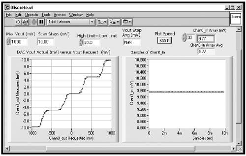
Figure A.16 shows the Front Panel of the VI Discrete.vi. This VI is for demonstrating the discrete nature of the sending and receiving functions. We first consider that of the sending function, as in the case of Discrete.vi in Fig. A.16
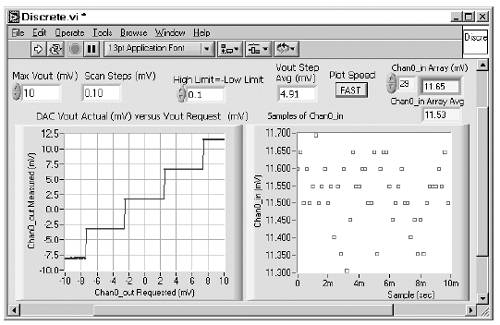
The graph on the left shows the voltage actually sent out (Y-axis) for a quasi-continuous range of requested (programmed) voltage to be sent out (X-axis). In the example, the program called for the output voltage to be swept over a range from -10 to 10 mV in steps of 100 mV. The actual voltage sent out is discrete in steps of 4.88 mV; thus only four steps over the entire range are sent out. The graph on the right is a plot of the input voltage samples from one (the last) measurement. The plot illustrates the inherent scatter in this type of measurement.
|
Project PA.6 Discrete Output Voltage from The DAQ |
In Fig. A.17 is shown the result of measuring a high-resolution output sweep with a less precision input mode of measurement. The high resolution is obtained with a resistance voltage divider. The graph on the left shows the discrete nature of the receiving function for a low-resolution mode. For the limit settings, the receiving resolution is 4.88 mV.
The transition regions are nonabrupt due, to the bit uncertainty (due to noise) in these regions. In Fig. A.18 is shown input voltage samples (for one output voltage) for a point in a plateau region (a) and for a point in the transition region (b). Note that the plot in the graph on the right in Fig. A.17 is for a plateau region (last point in the sweep in the plot on the left) and shows no scatter.
|
Project PA.7 Discrete Input Voltage from the Circuit Board |
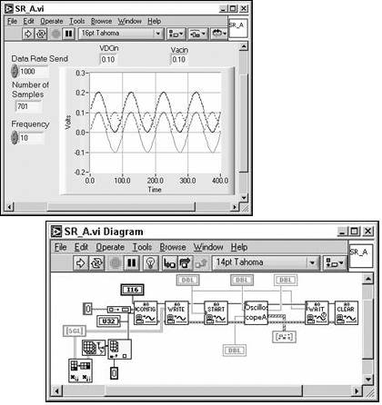
Measuring circuit response to waveform input signals requires simultaneous sending and receiving data with the DAQ. An example was demonstrated above with the oscilloscope measurement project (Fig. A.14). The function generator VI used for that measurement is FG_A.vi. The main subVI of the function generator VI is SR_A.vi. The Front Panel and Diagram of the VI are shown in Fig. A.19. The VI sends and receives voltage arrays from one output channel and one input channel.
Information supplied from the top VI, FG_A.vi, includes sine-wave (or square-wave) frequency (Frequency), number of cycles (Cycles), and number of samples per cycle (Samples/Cycle). The information is used to facilitate the computation Sample Rate = Frequency · Sample/Cycle and the size of the waveform data array (Cycle · Samples/Cycle).
The subVI, SR_A.vi, receives this information along with the waveform data array, as required by the functions in the Diagram of SR_A.vi (Fig. A.19). The waveform data array is calculated by a subVI, Sine-wave.vi (on the same level as SR_A.vi). (An alternative waveform, SquareWave.vi, is selectable from FG_A.vi). The execution sequence is AO Config.vi, AO Write.vi, AO Start.vi, OscilloscopeA.vi, AO Wait.vi, and AO Clear.vi.
The Number of Cycles is adjusted automatically in the top VI and increases for higher frequencies. The increase provides assurance that the outgoing waveform is still executing during the oscilloscope measurement phase. The duration of the waveform sent out is Cycles · T.
|
Project PA.8 Using the Simultaneous Sending/Receiving Function |
|
PA.1 |
Sending and Receiving Voltages with the Sending and Receiving VIs |
|
PA.2 |
Sending and Receiving Voltages from the Front Panel |
|
PA.3 |
Plotting Measured Samples |
|
PA.4 |
Using the Autoranging Voltmeter |
|
PA.5 |
Observing the Oscilloscope Output Graph |
|
PA.6 |
Discrete Output Voltage from the DAQ |
|
PA.7 |
Discrete Input Voltage from the Circuit Board |
|
PA.8 |
Using the Simultaneous Sending/Receiving Function |
|