ALTE DOCUMENTE
|
|||||
EXCEL 2000
Printed on: May 29, 2009

Table of Contents
What is Excel?
Creating or Opening Workbooks
Saving and Closing Workbooks
Moving Around in a Workbook
Arranging, Minimizing, and Hiding Windows
Basic Concepts and Skills
Aligning Sheet Data
Changing Column Widths and Row Heights
Enter a Formula
Plotting Data Series in Rows or Columns
The Default Chart Format
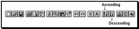
Volume/Hi-Lo-
Horizontal Gridlines
Sorting Data
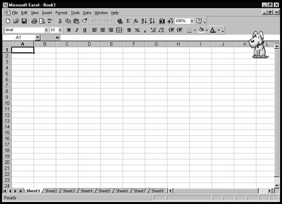
In Microsoft Excel, the file, in which you work and store your data, is called a workbook. Each workbook can contain many sheets. You can also have different types of sheets in one workbook.
For example, you could have a year's sales data on a sheet in a workbook, and also have a chart sheet for the data in the same workbook. Whenever you open, close, or save a file, you are opening, closing, or saving a workbook file.
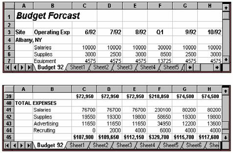
The default workbook opens with 3 sheets, named Sheet 1 through Sheet 3. The sheet names appear on tabs at the bottom of the workbook window. Move from sheet to sheet within a workbook by clicking on the tabs. The tab of the active sheet is always bold.
Active sheet tab
Note: If you do not see the tabs in the workbook, choose Options from Tools, select View, then select Sheet tabs
An Excel workbook contains sheets, charts, and/or macro sheets.
When Excel is started, Book 1 opens.
Ø 17317i84r ; 17317i84r ; 17317i84r ; 17317i84r ;
To create a
new book, click on New ![]()
Ø 17317i84r ; 17317i84r ; 17317i84r ; 17317i84r ; Or choose New from File to see the following dialog box.
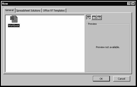
In this dialog box you have a choice to create a new Workbook or use the Spreadsheet Solutions tab.
Opening an Existing Workbook
Open a workbook recently worked on from the list at the bottom of File. If the list does not appear on File, choose Options from Tools; select the General tab and select Recently Used File List.
Ø 17317i84r ; 17317i84r ; 17317i84r ; 17317i84r ;
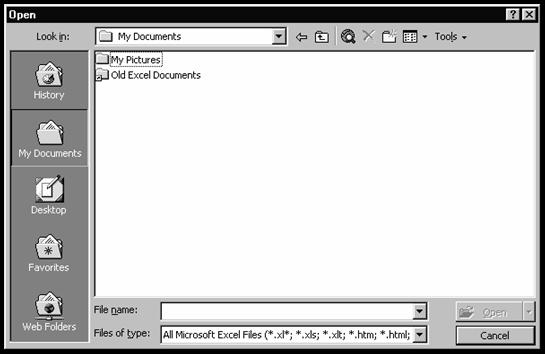
Open any
workbook by choosing Open from File or click on Open ![]() on the toolbar.
on the toolbar.
Ø 17317i84r ; 17317i84r ; 17317i84r ; 17317i84r ; Select a workbook.
Use the Look in: box to select a different drive, directory or folder to find a workbook.
Ø 17317i84r ; 17317i84r ; 17317i84r ; 17317i84r ;
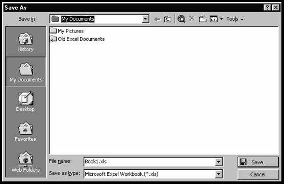
To save a
workbook, choose Save from File, or click on Save ![]() on the
toolbar.
on the
toolbar.
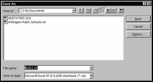
If you have not saved the workbook previously, or if it was opened as Read-Only, the Save As dialog box appears.
Ø 17317i84r ; 17317i84r ; 17317i84r ; 17317i84r ; Type a name for the workbook.
Ø 17317i84r ; 17317i84r ; 17317i84r ; 17317i84r ; Select the drive, directory, or folder where the workbook is to be saved.
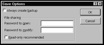
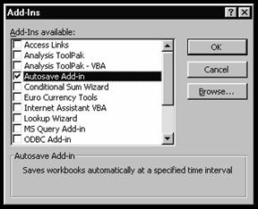
Ø 17317i84r ; 17317i84r ; 17317i84r ; 17317i84r ; To set up Excel so that it automatically saves your work, choose Add-ins from Tools and check AutoSave Add-in. Click on Ok
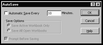
Ø 17317i84r ; 17317i84r ; 17317i84r ; 17317i84r ; Choose AutoSave from Tools and specify how often to save, what to save, and whether you should be prompted before saving.
|
|
Click a tab to select a sheet. |
![]()
![]()
![]()
![]()
![]()
|
Click to scroll the display of tabs to the right or left by a tab. To scroll by several tabs hold down Shift and click. |
Drag the tab split box left to see more of the scroll bar; drag right to see more tabs. Double-click to reset. |
The scrolling buttons only make different tabs visible; click on a tab to make a sheet active. Or use the keyboard to move from sheet to sheet.
Inserting Sheets
A new workbook opens with 3 sheets named Sheet 1 through Sheet 3. You can easily insert or delete sheets.
Tip: Change the number of sheets in a new workbook by choosing Options from Tools. Select the General tab and change the setting in the Sheets in new workbook box. The maximum number of sheets in a new workbook is 255.
Insert several sheets by holding down Ctrl and clicking on the number of sheets to be inserted, and choose Worksheet from Insert.
Deleting Sheets
Ø 17317i84r ; 17317i84r ; 17317i84r ; 17317i84r ; Select a sheet by clicking on the sheet tab.
Ø 17317i84r ; 17317i84r ; 17317i84r ; 17317i84r ; From Edit, choose Delete Sheet. The sheet to the right becomes the active sheet.
Ø 17317i84r ; 17317i84r ; 17317i84r ; 17317i84r ; Delete several sheets by holding down Ctrl while clicking on the sheets to be deleted, and choose Delete Sheet from Edit.
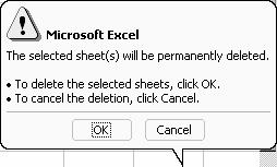
You will be warned that the sheet(s) will be permanently deleted. Click OK or Cancel.
Renaming Sheets
Rename any sheet up to 31 characters, including spaces.
Ø 17317i84r ; 17317i84r ; 17317i84r ; 17317i84r ; Double-click the tab of the sheet to be renamed. Type a new name in the dialog box.
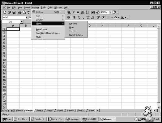
Ø 17317i84r ; 17317i84r ; 17317i84r ; 17317i84r ; You can also choose Sheet from Format and choose Rename.
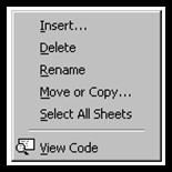
Ø 17317i84r ; 17317i84r ; 17317i84r ; 17317i84r ; Or right click the sheet and select Rename.
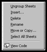
Sheets can be moved or copied within the same workbook, added to an existing workbook or put into a new workbook of its own.
Moving a Sheet WITHIN a Workbook
Ø 17317i84r ; 17317i84r ; 17317i84r ; 17317i84r ; Click and drag a sheet tab along the row of tabs, a black triangle indicates where the sheet will be moved.
Ø 17317i84r ; 17317i84r ; 17317i84r ; 17317i84r ; Release the mouse button and the sheet moves to the new location in the current workbook.
Ø 17317i84r ; 17317i84r ; 17317i84r ; 17317i84r ; Use Ctrl to select more than one sheet and drag the sheets to the new location. If the selected sheets are nonadjacent, the moved sheets are inserted together.
Adding a Sheet to an existing workbook
Ø 17317i84r ; 17317i84r ; 17317i84r ; 17317i84r ; Select the sheet or sheets to be added.
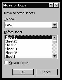
Ø 17317i84r ; 17317i84r ; 17317i84r ; 17317i84r ; Choose Move or Copy Sheet from Edit.
Ø 17317i84r ; 17317i84r ; 17317i84r ; 17317i84r ; Select the destination workbook and where the sheets are to be placed. The sheets are moved to the selected workbook.
Ø 17317i84r ; 17317i84r ; 17317i84r ; 17317i84r ; Or, use the right mouse button to choose Move or Copy...

Notes: If a sheet with the same name exists in the destination workbook the moved sheet will be renamed with a number in sequence with its creation in parentheses.
Sheets can also be moved between workbooks by dragging the sheet tabs across workbook windows. Arrange the workbook windows so that the sheet tabs for both workbooks are visible before dragging.
Moving a Sheet into a NEW Workbook
Ø 17317i84r ; 17317i84r ; 17317i84r ; 17317i84r ; Choose Move or Copy Sheet from Edit to move sheets into a new workbook.
Ø 17317i84r ; 17317i84r ; 17317i84r ; 17317i84r ; Select New Book as the destination workbook in the To Book box. A new workbook will contain only the selected sheets.
Ø 17317i84r ; 17317i84r ; 17317i84r ; 17317i84r ; Or drag sheets outside of a workbook window and release the mouse button.
Copying a Sheet WITHIN a Workbook
When copying sheets within a workbook, Excel renames the copy of the sheet.
For example, a copy of Sheet 1 becomes Sheet 1
Ø 17317i84r ; 17317i84r ; 17317i84r ; Select the sheet, press Ctrl, and drag the sheet along the row of tabs. A black triangle indicates where a copy of the sheet will be inserted.
Ø 17317i84r ; 17317i84r ; 17317i84r ; Release the mouse button and the sheet is copied to the new location.
Ø 17317i84r ; 17317i84r ; 17317i84r ; 17317i84r ; Use Ctrl to select more than one sheet and drag the sheets to the new location. If the selected sheets are nonadjacent, the copied sheets are inserted together.
Adding a Copied Sheet to ANOTHER Workbook
Ø 17317i84r ; 17317i84r ; 17317i84r ; Select the sheet or sheets to be copied.
Ø 17317i84r ; 17317i84r ; 17317i84r ; Choose Move Or Copy Sheet from Edit.
Ø 17317i84r ; 17317i84r ; 17317i84r ; Select the destination workbook and select the Create A Copy check box. The sheets are copied to the selected workbook. If the selected sheets are nonadjacent, the copied sheets are inserted together.
Ø 17317i84r ; 17317i84r ; 17317i84r ; 17317i84r ; Or, use the right mouse button to choose Move or Copy...
![]()
Ø 17317i84r ; 17317i84r ; 17317i84r ; 17317i84r ; If this is a copy click on Create a copy
Copying a Sheet into a New Workbook
Ø 17317i84r ; 17317i84r ; 17317i84r ; Choose Move or Copy Sheet. from Edit to copy sheets into a new workbook.
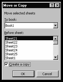
Ø 17317i84r ; 17317i84r ; 17317i84r ; Click on the drop down list in the To book: box. Select (new book) as the destination workbook in the To Book: box and select the Create a copy check box. A new workbook is created that contains only the selected sheets.
Ø 17317i84r ; 17317i84r ; 17317i84r ; Or hold down Ctrl and drag the sheets outside the workbook window and release the mouse button.
Opening, Arranging, and Closing Workbook Windows
Multiple windows make it easy to enter, compare, format, and edit data in:
Ø 17317i84r ; 17317i84r ; 17317i84r ; 17317i84r ; Different parts of a sheet
Ø 17317i84r ; 17317i84r ; 17317i84r ; 17317i84r ; Different sheets in the same workbook
Ø 17317i84r ; 17317i84r ; 17317i84r ; 17317i84r ; Two or more workbooks
Create a new window on a workbook by choosing New Window from Window. Arrange the windows to see them all at the same time.
Windows showing different parts of one sheet
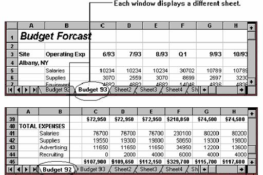
Windows showing different sheets in the same workbook
Windows showing different workbooks
To move around in the different windows, click a window or choose its name from the Window menu. A window can be closed, hidden, or minimized when it is no longer needed.
Arrange multiple windows to see them all by choosing Arrange. from Window.
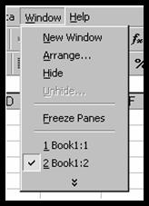
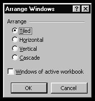
Ø 17317i84r ; 17317i84r ; 17317i84r ; 17317i84r ; To arrange only the windows of the active workbook, select the Windows of active workbook check box in the Arrange Windows dialog box.
Hide windows by switching to the window you want to hide and choose Hide from Window. Hidden windows remain open. Unhide windows by choosing Unhide from Window and select the windows to unhide in the dialog box. You can minimize windows so that they appear as a workbook icon in the Excel workspace. These icons can be arranged on the screen, or restored by double clicking.
Closing Windows
When a window is no longer needed, close the window, by double-clicking the workbook Control-menu box, or choose Close from the workbook Control menu.
If the window is the only window of the workbook, the workbook will be closed when the window is closed. If changes have been made since the workbook was last saved, a prompt appears to save changes.
Excel offers several ways to choose commands:
Ø 17317i84r ; 17317i84r ; 17317i84r ; 17317i84r ; From the menu bar
Ø 17317i84r ; 17317i84r ; 17317i84r ; 17317i84r ; From shortcut menus that can be displayed by clicking with the right mouse button.
Ø 17317i84r ; 17317i84r ; 17317i84r ; 17317i84r ; By clicking tools on the toolbar with the mouse
Ø 17317i84r ; 17317i84r ; 17317i84r ; 17317i84r ; By using the keyboard
Choose Commands from the Menu
Excel commands are grouped into menus across the menu bar displayed across the top of the application window. Different document types have different menu bars.
For example, if working in a separate chart, you will see the chart menu bar.
Some
commands display a sub-menu. Sub-menus
are indicated by a![]() following the command name. Sub-menus contain additional, related
commands.
following the command name. Sub-menus contain additional, related
commands.
When a command name followed by an ellipsis ( is chosen, Excel displays a dialog box so you can enter more information or select options before carrying out the command.
The following illustration shows the commands on the File menu:
Some command names occasionally appear
dimmed which indicates that the command does not apply to the current situation
or that a selection must be made or an action completed before choosing the
command.
Shortcut Menus
Shortcut menus are displayed by using the right mouse button. Shortcut menus contain the most useful commands for the cell, chart, or other selected objects. If you can edit or format something in Excel, you can probably use a shortcut menu to do so.
Select a command from the menu, or click outside the menu to close it.
Ø 17317i84r ; 17317i84r ; 17317i84r ; 17317i84r ; Place the cursor/arrow on a toolbar.
Ø 17317i84r ; 17317i84r ; 17317i84r ; 17317i84r ; Click the right mouse button. Select another toolbar.
Ø 17317i84r ; 17317i84r ; 17317i84r ; 17317i84r ; Click outside the shortcut menu to close, or press Esc.
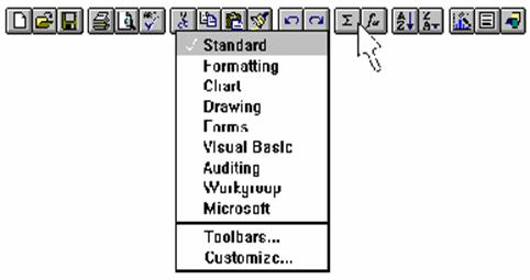
Toolbars
Excel includes a set of toolbars designed to perform frequent tasks quickly or work on specific activities, such as charting, more efficiently. Each toolbar contains tools that you select to carry out commands or other actions. Just like menu commands, some tools carry out an immediate action, while others require additional action, such as drawing.
Ø 17317i84r ; 17317i84r ; 17317i84r ; 17317i84r ; To see a description of a tool without invoking it, point to the tool while holding down the mouse button. A brief description of that tool appears in the status bar.
Ø 17317i84r ; 17317i84r ; 17317i84r ; 17317i84r ; To select the tool, release the mouse button.
Ø 17317i84r ; 17317i84r ; 17317i84r ; 17317i84r ; To cancel the tool, move the pointer off the tool and release the mouse button.
 |
Cells
The Cell is the basic unit of the spreadsheet. Text, numbers, or formulas can be stored in a cell. The amount of data stored in a cell is not limited by the size of the cell on the screen. A column letter and row number identifies each cell. The current cell (the one in which the cursor is positioned) appears with a dark border. This is the cell in which anything you type will be stored or which will be affected by any command or function selected.
Rows and Columns
Columns are labeled with letters, starting at A through Z and continue with double-letter names, AA through AZ, BA through BZ, etc. The final column is IV for a total of 256 available columns. Rows are labeled from 1 to 65,536.
Using the mouse, move the pointer to a cell and click once. It may be necessary to use the scroll bars to move the view to a screen that displays that cell.
Using the menu, select Edit and then the GoTo command. A dialog box appears in which you can type the cell address (column letter and row number) to go to the cell.
Use the arrows to move from cell to cell. PgUp and PgDn will move the view up or down one screen. Ctrl+Home will move to cell A1 in the upper left-hand corner of the spreadsheet.
Select Groups of Cells
Many functions can be performed on more than one cell at a time.
Ø 17317i84r ; 17317i84r ; 17317i84r ; 17317i84r ; To select a range of cells, position the pointer on the cell in one corner of the group you wish to indicate.
Ø 17317i84r ; 17317i84r ; 17317i84r ; 17317i84r ; Press and drag the mouse until the selected area on the screen includes all the cells you want in this range.
Ø 17317i84r ; 17317i84r ; 17317i84r ; 17317i84r ; If you have released the mouse button and wish to add cells to the range, hold down Shift and continue to drag the highlighted areas to include additional cells.
Ø 17317i84r ; 17317i84r ; 17317i84r ; 17317i84r ; If you wish to include cells that are not adjacent to the existing range, hold down Ctrl and proceed to select an additional group of cells.
Ø 17317i84r ; 17317i84r ; 17317i84r ; 17317i84r ; To de-select a range, move the pointer to a cell not in the range and click.
Select Columns or Rows
Ø 17317i84r ; 17317i84r ; 17317i84r ; 17317i84r ; To apply a command to all of the cells in a particular column or row, click on a column or row heading. All cells in that column or row will be highlighted.
Ø 17317i84r ; 17317i84r ; 17317i84r ; 17317i84r ; To select more than one column or row, click & drag the mouse across the headers of the columns or rows.
Create a Sheet
The spreadsheet, is the primary document used to store and manipulate data. A sheet is displayed in a window that can be moved and sized like any other window. This allows you to view more than one sheet window in the workspace at the same time.
Entering Data
A constant value is data typed directly into a cell; it can be a numeric value, including a date or time, or it can be text.
A formula is a sequence of constant values, cell references, names, functions or operators that produce a new value. Formulas always begin with an equal sign (=).
Constant values do not change unless you select the cell and edit the value yourself. A value that is produced as the result of a formula can change when other values in the sheet change.
You can enter three basic types of constant values: numbers, dates and times (which are stored as numbers) and text. Use the formula bar to enter values in sheet cells.
Enter data in a cell by selecting the cell and typing. You can also enter data in a cell range.
Select the range of cells. You can then make cell entries, one after another, in successive cells in the range by pressing Enter to move to the next cell after you finish typing.
You can also make non-adjacent selections and enter data into the selected cells. Non-adjacent selections are made up of single cells or ranges that are not next to each other. You can make cell entries, one after another, without first moving to the next cell or cell range.
To create a new workbook:
Ø 17317i84r ; 17317i84r ; 17317i84r ; 17317i84r ;
Click on New ![]() , on the Standard toolbar, or choose New from File.
, on the Standard toolbar, or choose New from File.
Ø 17317i84r ; 17317i84r ; 17317i84r ; 17317i84r ; Select New, General, Workbook, OK. Excel displays a new Book.
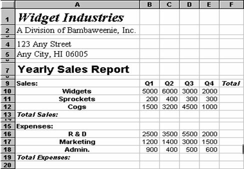
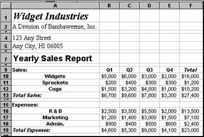
Pretend we are the CEO of Widget Industries, a division of Bambaweenie, Inc. As the CEO of a small and upcoming company we are going to generate a yearly report.
Ø 17317i84r ; 17317i84r ; 17317i84r ; 17317i84r ; Select cell A1. Type Widget Industries. Press Enter. Widget Industries will stretch across more than one column.
Finish up the spreadsheet to match this:
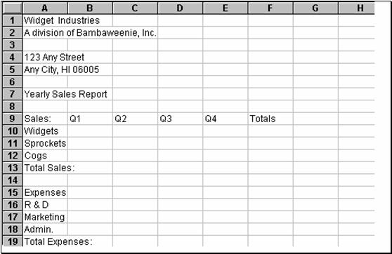
Notice that the title is longer than the cell in which it was typed, but the entire text is displayed on the screen. This only occurs if there is no data in the cell to the right. At this point, many of the column headings overlap and are unreadable.
Ø 17317i84r ; 17317i84r ; 17317i84r ; 17317i84r ; Save the document as a:Widget Industries Yearly Sales Report.xls.
Editing a Cell using the mouse
Edit a cell in your sheet by typing a new entry over an existing one, or edit part of the information within the cell. You can also edit a cell's contents in the formula bar. Use the same techniques to edit within a cell and in the formula bar.
Ø 17317i84r ; 17317i84r ; 17317i84r ; 17317i84r ; To position the insertion point in the cell, point and click.
Ø 17317i84r ; 17317i84r ; 17317i84r ; 17317i84r ; To edit within a cell, double-click the cell. The insertion point appears and you can edit the cell's formula or value.
Ø 17317i84r ; 17317i84r ; 17317i84r ; 17317i84r ; To select characters in the cell drag through the characters with the mouse while holding the left mouse button down.
Ø 17317i84r ; 17317i84r ; 17317i84r ; 17317i84r ; To select a word in the cell, double-click the word you want.
Editing a Cell using the menu
From Edit use Cut, Copy, and Paste.
Ø 17317i84r ; 17317i84r ; 17317i84r ; 17317i84r ; Cut removes the selected characters from the cell and places them on the Clipboard.
Ø 17317i84r ; 17317i84r ; 17317i84r ; 17317i84r ; Copy makes a copy of the selected characters and places them on the Clipboard.
Ø 17317i84r ; 17317i84r ; 17317i84r ; 17317i84r ; Paste inserts the contents of the Clipboard in a cell at the insertion point.
Ø 17317i84r ; 17317i84r ; 17317i84r ; 17317i84r ; Clear removes the selected characters from the cell. The characters are not stored on the Clipboard.
Ø 17317i84r ; 17317i84r ; 17317i84r ; 17317i84r ; Delete also clears selected characters and does not store them on the clipboard.
Moving and Copying Cells
Change the location of cells on a sheet by copying or moving cells to a different part of the same sheet, to another workbook, or to another application. Use Cut, Copy and Paste or drag the mouse.
When a cell is copied, it is duplicated and can be pasted into a new location. When a cell is moved, the cell contents are removed and pasted into a new location. Cells that are copied or moved can be inserted between existing cells, or pasted over the existing cell contents.
When cells are copied, references in the original cells are not affected. Excel adjusts relative references of formulas that are pasted into new locations. When cells are moved, Excel adjusts relative references to the moved cells to reflect their new locations.
Move or copy characters within a cell
Ø 17317i84r ; 17317i84r ; 17317i84r ; 17317i84r ; Double-click the cell you want to edit.
Ø 17317i84r ; 17317i84r ; 17317i84r ; 17317i84r ; In the cell, select the characters you want to move or copy.
Ø 17317i84r ; 17317i84r ; 17317i84r ; 17317i84r ; To move the characters, click Cut.
Ø 17317i84r ; 17317i84r ; 17317i84r ; 17317i84r ; To copy the characters, click Copy.
Ø 17317i84r ; 17317i84r ; 17317i84r ; 17317i84r ; In the cell, click where you want to paste the characters.
Ø 17317i84r ; 17317i84r ; 17317i84r ; 17317i84r ; Click Paste.
Moving and Copying Cells with Cut, Copy and Paste
Use Cut, Copy and Paste commands, toolbar buttons, or shortcut keys if copying or moving cells long distances within a large sheet, to a different sheet within a workbook, or to another window or application.
When cells are moved, they are cut and transferred to another location.
To move cells with Cut and Paste:
Ø 17317i84r ; 17317i84r ; 17317i84r ; 17317i84r ; Select the cell or cells to be moved.
Ø 17317i84r ; 17317i84r ; 17317i84r ; 17317i84r ; From Edit, choose Cut. The cut area is marked with a moving border. Excel moves the data to the Clipboard.
Ø 17317i84r ; 17317i84r ; 17317i84r ; 17317i84r ; To move the data to another sheet, switch to that sheet.
Ø 17317i84r ; 17317i84r ; 17317i84r ; 17317i84r ; From Edit, choose Paste.
In addition to pasting the contents of the Clipboard at the insertion point in a cell, you can paste them into a blank cell, into a formula in another cell, or to replace selected text.
Note: Undo or repeat most editing actions and commands by clicking Undo or Repeat immediately after performing an action or choosing a command.
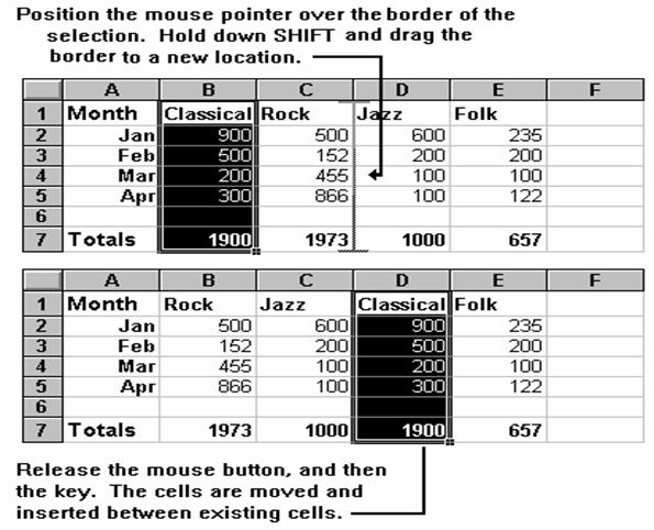
Moving Cells by Dragging
Ø 17317i84r ; 17317i84r ; 17317i84r ; 17317i84r ; Position the mouse pointer over the border of a selection and drag the border to a new location.
Ø 17317i84r ; 17317i84r ; 17317i84r ; 17317i84r ; While dragging, the border appears to indicate the size and position of the selection. If the area is located beyond the visible portion of the sheet, drag the selection to the edge of the window to scroll through the sheet.
Ø 17317i84r ; 17317i84r ; 17317i84r ; 17317i84r ; Position the border so that it is surrounding the area. The pointer must be inside a cell in the area. Release the mouse button. When you move cells that contain data, the old cells are replaced with the moved cells.
Insert moved or copied cells between existing cells
Ø 17317i84r ; 17317i84r ; 17317i84r ; 17317i84r ; Select the cells that contain the data you want to move or copy.
Ø 17317i84r ; 17317i84r ; 17317i84r ; 17317i84r ; To move the selection, click Cut.
Ø 17317i84r ; 17317i84r ; 17317i84r ; 17317i84r ; To copy the selection, click Copy.
Ø 17317i84r ; 17317i84r ; 17317i84r ; 17317i84r ; Select the upper-left cell where you want to place the cut or copied cells.
Ø 17317i84r ; 17317i84r ; 17317i84r ; 17317i84r ; On the Insert menu, click Cut Cells or Copied Cells.
Ø 17317i84r ; 17317i84r ; 17317i84r ; 17317i84r ; Click the direction you want to shift the surrounding cells.
Note: To cancel the moving border after you finish copying, press ESC.
Inserting Cells by Dragging
To insert copies of cells, press Ctrl+Shift and then drag the border.
To move or insert cells between cells by dragging:
Ø 17317i84r ; 17317i84r ; 17317i84r ; 17317i84r ; Select the cell or cells to be moved. Position the mouse pointer over the border. The mouse pointer changes to an arrow.
Ø 17317i84r ; 17317i84r ; 17317i84r ; 17317i84r ; Hold down Shift and drag the border to the row or column gridline where you want to insert the data. If the paste area is located beyond the visible portion of the sheet, drag the selection to the edge of the window to scroll through the sheet.
Ø 17317i84r ; 17317i84r ; 17317i84r ; 17317i84r ; Release the mouse button first then the shift key. If you release shift, then the mouse button, it will replace the information in the cell to the right of the insertion point. The selection is inserted between the cells bordering the row or column gridline.
Using the Shortcut Menu When Dragging
Copying cells duplicates the cells and pastes them into another location - either on the same sheet or on a different sheet. When cells are copied, Excel copies the cell contents, the cell formats, and any notes attached to the cell. You can choose to paste all or only one of these attributes into the new location, or paste area, using Paste Special.
Designate the paste area in the same way that you do when you are moving cells. Select either a single cell to designate the upper-left corner of the paste area, or select an area the same size and shape as the copied area. Excel automatically adjusts relative references in the paste area. The relative references refer to cells relative to the paste area instead of to cells relative to the original copied cells.
Ø 17317i84r ; 17317i84r ; 17317i84r ; 17317i84r ; Select the cells to be copied and choose Copy from Edit. The copy area is marked with a moving border.
Ø 17317i84r ; 17317i84r ; 17317i84r ; 17317i84r ; Choose Paste from Edit. The destination cell becomes the upper-left corner of the paste area. The moving border indicates that you can paste the copied cells again.
Ø 17317i84r ; 17317i84r ; 17317i84r ; 17317i84r ; To cancel the border, press Esc.
To copy and replace cells with the Cut and Paste commands:
Ø 17317i84r ; 17317i84r ; 17317i84r ; 17317i84r ; Select the cell or cells to copy. Choose Copy from Edit. A moving border marks the copy area. To copy the cells to another sheet, switch to the other sheet.
Ø 17317i84r ; 17317i84r ; 17317i84r ; 17317i84r ; From Edit, choose Paste.
Ø 17317i84r ; 17317i84r ; 17317i84r ; 17317i84r ; To copy the same cells to another location, repeat the last steps.
Ø 17317i84r ; 17317i84r ; 17317i84r ; 17317i84r ; To cancel the moving border after copying, press Esc.
Ø 17317i84r ; 17317i84r ; 17317i84r ; 17317i84r ; To shift the cells in the paste area right, select Shift Cells Right.
Ø 17317i84r ; 17317i84r ; 17317i84r ; 17317i84r ; To shift the cells in the paste area down, select Shift Cells Down. Choose OK.
Pasting Multiple Copies
You can paste copied cells in many areas of the sheet by selecting the upper left cell of the paste area, pasting the cells, and repeating these steps to make multiple copies. You can also paste multiple copies of a cell or range on a sheet using one paste operation.
Ø 17317i84r ; 17317i84r ; 17317i84r ; 17317i84r ; Select the cell or cells to be copied. From Edit, choose Copy, Excel surrounds the selection with the moving border.
Ø 17317i84r ; 17317i84r ; 17317i84r ; 17317i84r ; From Edit, choose Paste. To paste multiple copies in nonadjacent areas on the sheet, hold down Ctrl as you make additional selections.
Ø 17317i84r ; 17317i84r ; 17317i84r ; 17317i84r ; To cancel the moving border after copying, choose a command, switch to the formula bar, or press Esc.
Copying Cells by Dragging
Position the mouse pointer over the border of a selection. Hold down Ctrl and drag the border to a new location. Release the mouse button, and then the key. The cell contents are copied to their new location. When you copy over cells that contain data, the old cells are replaced with the copied cells.
To copy and insert cells between existing cells by dragging:
Ø 17317i84r ; 17317i84r ; 17317i84r ; 17317i84r ; Position the mouse pointer over the border of the selection. The mouse pointer changes to an arrow.
Ø 17317i84r ; 17317i84r ; 17317i84r ; 17317i84r ; Press Ctrl+Shift and drag the selection to the row or column gridline where you want to copy and insert the selection. If the paste area is located beyond the visible portion of the sheet, drag the selection to the edge of the window to scroll through the sheet. Release the mouse button. The cells are moved and inserted between existing cells.
To insert copied cells between existing cells with the Insert command:
Ø 17317i84r ; 17317i84r ; 17317i84r ; 17317i84r ; Select the cell or cells to be copied.
Ø 17317i84r ; 17317i84r ; 17317i84r ; 17317i84r ; From Edit, choose Copy, Excel surrounds the selection with the moving border. If you want to copy the cells to another sheet, switch to the other sheet.
Ø 17317i84r ; 17317i84r ; 17317i84r ; 17317i84r ; To insert copied cells choose Copied Cells or Cut Cells from Insert or Insert Cut Cells or Insert Copied Cells from the shortcut menu.
Ø 17317i84r ; 17317i84r ; 17317i84r ; 17317i84r ; To cancel the moving border, press Esc.
Note: Insert cells once after each copy. To insert cells again, repeat the procedure.
Inserting, Deleting and Clearing Cells, Rows and Columns
You can insert, delete, or clear cells, rows or columns to change the structure of data on a sheet. You can insert blank cells or entire blank rows and columns anywhere on a sheet. When you insert cells, the other cells on the sheet are shifted to make room for the new cells. When you delete cells, the surrounding cells shift to fill in the space. When you clear cells, only the cell contents are removed; the empty cells remain.
Inserting Rows or Columns
When you insert a row or column, Excel creates a new blank row or column and shifts the existing rows and columns to make room for the inserted cells. Excel will adjust the references to the shifted cells to reflect their new locations.
Ø 17317i84r ; 17317i84r ; 17317i84r ; 17317i84r ; Select the number of rows you want to shift to open space for new rows.
Ø 17317i84r ; 17317i84r ; 17317i84r ; 17317i84r ; Choose Rows from Insert; new blank rows are inserted above the selection.
Follow the same steps to insert columns.
Ø 17317i84r ; 17317i84r ; 17317i84r ; 17317i84r ; Select the number of columns you want to shift to open space for new columns, and then choose Columns from Insert.
When you insert columns, the new blank columns are placed to the left of the selected columns.
Inserting Blank Cells
Ø 17317i84r ; 17317i84r ; 17317i84r ; 17317i84r ; Select a range of cells the same size as the new cells you want to insert. From Insert choose cells.
Ø 17317i84r ; 17317i84r ; 17317i84r ; 17317i84r ; In the Insert dialog box, select Shift Cells Right or Shift Cells Down to shift the other cells in the sheet to accommodate the inserted cells.
Ø 17317i84r ; 17317i84r ; 17317i84r ; 17317i84r ; Choose OK. New blank cells are inserted.
Deleting Cells Vs Clearing Cells
Clearing and deleting are two ways to remove data from an Excel document.
Clearing a cell clears the contents, formats, or notes - or all three - from that cell, but leaves the cleared cell in the structure of the sheet.
Deleting a cell completely removes the cell and its notes from the sheet and moves adjacent cells to close up the space that was occupied by the deleted cell.
Clearing and deleting cells produce different results for formulas that reference those cells. If a cell is cleared, its value is zero; a formula referring to that cell will get a value of zero from that cell. If a cell is deleted, it no longer exists; a formula referring to the deleted cell will not be able to find it and will return the #REF! error value.
For example, enter the formula =A1*B1 in a cell and then clear cell B1, the result of the formula will be zero (A1*0). If you delete cell B1, the cell containing the formula =A1*B1 is changed to =A1*#REF! and produces the #REF! error value to let you know to adjust your formula.
Always use caution when deleting cells. However, if a cell is inadvertently cleared or deleted, restore it by immediately choosing Undo from Edit before doing anything else on the sheet. Notes attached to deleted cells are deleted with the cells; notes that belong to moved cells follow the cells to their new locations.
Deleting Cells
Ø 17317i84r ; 17317i84r ; 17317i84r ; 17317i84r ; Select the range of cells to be deleted.
Ø 17317i84r ; 17317i84r ; 17317i84r ; 17317i84r ; From Edit, choose Delete. In the Delete dialog box, select the direction you want the surrounding cells to move. The selected cells are deleted.
Clearing Cells
Ø 17317i84r ; 17317i84r ; 17317i84r ; 17317i84r ; Select the cells you want to clear. When you press Delete, the cell contents are cleared and cells remain.
You can also clear cells by selecting them, choosing Clear from Edit, and then selecting All, Contents, Formats, or Notes. Clearing the contents clears any formulas or data from a cell.
Filling Adjacent Cells and Creating Series
Copy contents of cells into other cells by dragging the fill handle, the black square located in the lower-right corner of the selection. Or, use Fill from Edit.
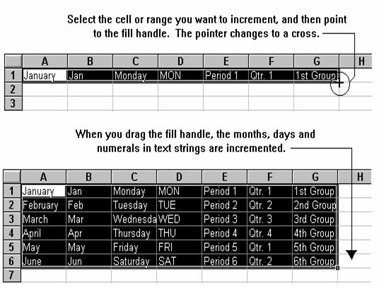
Create a series by incrementing the value in the active cell into a range by dragging the fill handle. The fill handle copies and fills data, and creates a series using AutoFill. Drag the fill handle to the left, right, up or down to fill data.
Dragging to Fill a Range
Ø 17317i84r ; 17317i84r ; 17317i84r ; 17317i84r ; Select the cell or cells and then point to the fill handle. The pointer changes to a black cross.
Ø 17317i84r ; 17317i84r ; 17317i84r ; 17317i84r ; Drag the fill handle in the direction to be filled. When the mouse is released, the data is filled into the range.
Tip: Select the range, type the data, and press Ctrl+Enter.
Caution: If you drag the fill handle up or to the left of a selection and stop in the selected cells without going past the first column or the top row, you will erase the data within the selection.
Double-Clicking To Fill a Range
Fill a range adjacent to a range of data by double-clicking the fill handle. Double-clicking the fill handle extends the selection from the current cell to the row at the end of the adjacent range and fills data into the selection.
Incrementing a Series of Numbers or Dates
When you drag the fill handle in a cell or range of cells that contain values that Excel recognizes as a series of sequential numbers, the series is incremented in the range you drag through. Some examples of data types and their sequences are listed in the following table:
|
Data Type |
Initial Selection |
Extended Series |
|
Numbers |
||
|
Months and Dates |
Jan |
Feb, Mar, Apr, May,... |
|
Ordinals |
1st Period |
2nd Period, 3rd Period, 4th Period,... |
Enter the values 5, 10, and 15 into 3 consecutive cells. Excel determines the series to be increments of 5 and enters 20, 25 into adjacent cells when the fill handle is dragged. If a group is selected, use Fill on Edit to copy the selection to the same location on all other sheets in the group.
You can also choose Fill from Edit, and then Series to increment series.
Creating a Series Based on a Single Value
Creating a Series Based on Multiple Values
Controlling How Values Are Incremented
Use Ctrl both to create a series from simple values and to suppress series that Excel normally increments. If the active cell contains a simple value, such as 40, the value is copied into the range you drag through.
Ø 17317i84r ; 17317i84r ; 17317i84r ; 17317i84r ; To increment a simple value through a range, for example to increment 40 to 41, 42, 43 and so on, hold down Ctrl and then drag the fill handle.
Ø 17317i84r ; 17317i84r ; 17317i84r ; 17317i84r ; To prevent values that Excel automatically increments, such as Jan and Qtr1, from incrementing, hold down Ctrl and then drag the fill handle.
Creating a Series That Decreases in Value
Ø 17317i84r ; 17317i84r ; 17317i84r ; 17317i84r ; To create a series that decreases in value, drag the fill handle up or to the left.
For example, if you have a series such as 0, 1, 2 that extends right, you could extend the series left for -3, -2, -1, 0, 1, and 2.
Caution: If you drag the fill handle up or to the left of a selection and stop in the selected cells without going past the first column or the top row, you will erase the data within the selection.
Filling Cells, Values, and Formats Using the Shortcut Menu
Ø 17317i84r ; 17317i84r ; 17317i84r ; 17317i84r ; Choose commands for filling data from the AutoFill shortcut menu after dragging the fill handle.
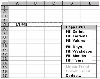
Ø 17317i84r ; 17317i84r ; 17317i84r ; 17317i84r ; To display the shortcut menu, drag the fill handle while holding down the right mouse button. Or, use Fill on Edit to fill data into adjacent cells in a selection.
Finding and Replacing Text, Numbers, or Cells
You can find cells that contain specific characters on a sheet by choosing Find from Edit.
Ø 17317i84r ; 17317i84r ; 17317i84r ; 17317i84r ; To find and replace sequences of characters in cells, choose Replace from Edit. These commands can be used on all sheets except Visual Basic modules.
Tip: To find and replace characters on more than one sheet, select a group of sheets and choose Replace from Edit. To find and replace data on all sheets in a workbook, choose Select All Sheets from the sheet tab shortcut menu. Choose Replace from Edit.
Finding Cells with Specific Types of Contents
Use the Go To Special dialog box to find and select cells with specific types of contents, such as constant values, formulas, notes, or blanks.
Ø 17317i84r ; 17317i84r ; 17317i84r ; 17317i84r ; To find and select cells with specific types of contents, choose Go To from Edit, choose the Special button, and then select the option you want.
Ø 17317i84r ; 17317i84r ; 17317i84r ; 17317i84r ; Press Tab and Shift+Tab to move through selected cells.
Ø 17317i84r ; 17317i84r ; 17317i84r ; 17317i84r ; Press Ctrl+Alt+ or Ctrl+Alt+ to move between areas of a nonadjacent selection.
Formatting Your Data for the Look You Want
With Excel, change the appearance of data in your sheet by changing the font, size, style, and color of data in a cell, text box, or button.
Format numbers to designate dollar amounts, percentages, decimals, scientific notations, dates, or times. Excel includes many built-in formats, or you can create your own formats to suit your specific needs. Format cells that contain data, as well as blank cells. When the data is entered into the formatted blank cells, Excel automatically formats the data.
When working with sheets that are similar in organization, save time by selecting these sheets as a group. The formatting you apply in the active sheet is automatically duplicated in the same location in all the sheets in the group.
All formatting options are available with the commands on the Format menu, by selecting Cells then Font or Number tabs. The most frequently used formatting options are also provided as tools on the Standard or Formatting toolbars.
Applying Formats
Autoformats and styles make it easy to apply combinations of formats.
Autoformats Apply combinations of built-in formats to ranges of data with AutoFormat on Format. The Autoformat command recognizes text, values, and formulas in the current range, and applies formats accordingly.
Styles Use styles to save combinations of cell formats and apply them to other cells and ranges. When you change the formats for a cell style, all cells using that style are updated to reflect the change.
Copying Formats
Use
Format Painter ![]() to quickly copy
formats from a cell and apply that cell's formats to another cell or range of
cells. Click the cell containing the
formats you want to copy, and then click Format Painter and drag through the range where you want to apply
the formats.
to quickly copy
formats from a cell and apply that cell's formats to another cell or range of
cells. Click the cell containing the
formats you want to copy, and then click Format Painter and drag through the range where you want to apply
the formats.
To change the appearance of data with the formatting tools:
Ø 17317i84r ; 17317i84r ; 17317i84r ; 17317i84r ; Select the cell or range of cells to be formatted.
A format change applies to the entire contents of a cell; you cannot format individual characters within the cell. Individual characters in a text box or button, however can be formatted.
Ø 17317i84r ; 17317i84r ; 17317i84r ; 17317i84r ;
To format
cell entries as bold or italic,
click on ![]() or
or ![]() on the Format toolbar.
on the Format toolbar.
Ø 17317i84r ; 17317i84r ; 17317i84r ; 17317i84r ; To change the font or the size of a cell entry, click the down arrows on the Font box or Font Size box.
Ø 17317i84r ; 17317i84r ; 17317i84r ; 17317i84r ;
![]() The tools are on the Formatting toolbar.
The tools are on the Formatting toolbar.
To change the appearance of data with the Font command:
Ø 17317i84r ; 17317i84r ; 17317i84r ; 17317i84r ; Select the cell, range, or entire sheet to be formatted.
Ø 17317i84r ; 17317i84r ; 17317i84r ; 17317i84r ; From Format choose Cells, and the Font tab; or on the shortcut menu, choose Format cells and the Font tab.
Ø 17317i84r ; 17317i84r ; 17317i84r ; 17317i84r ; Under Format, choose Cells, Size, and select a size from the list. If the size is not listed, type the size in the Size box. If the size is not available on the printer, another size may be substituted when you print the document.
Ø 17317i84r ; 17317i84r ; 17317i84r ; 17317i84r ; Select any other style effects and choose OK.
Ø 17317i84r ; 17317i84r ; 17317i84r ; 17317i84r ; Select cell A1. Choose Format, Cells then the Font tab.
Ø 17317i84r ; 17317i84r ; 17317i84r ; 17317i84r ; Make the font Times New Roman, Size 20, Bold Italic. Click on OK.
Ø 17317i84r ; 17317i84r ; 17317i84r ; 17317i84r ; Select cell A2, A4 and A5
Ø 17317i84r ; 17317i84r ; 17317i84r ; 17317i84r ; Choose Times New Roman, Size 12 from Font and Font Size on the Formatting bar.
Ø 17317i84r ; 17317i84r ; 17317i84r ; 17317i84r ;
Select cell A7. Choose font size 16 from the Font Size box on the Formatting toolbar; click on![]() .
.
Ø 17317i84r ; 17317i84r ; 17317i84r ; 17317i84r ;
Select cells A9 through A13. Hold down Ctrl. Select cells A15 through A19. Select cells B9 through F9 click on![]() .
.
Ø 17317i84r ; 17317i84r ; 17317i84r ; 17317i84r ;
Select cells F9, A13, and A19, click on![]() .
.
Select the alignment you want for the numbers or characters in sheet cells. Unless you change the alignment, all cells initially have the General format, which automatically aligns numbers to the right, text to the left and logical and error values centered. The easiest way to align the contents of cells is to use the buttons on the Formatting toolbar.
Ø 17317i84r ; 17317i84r ; 17317i84r ; 17317i84r ; Select the cell, range, text boxes, buttons, or the entire sheet you want to format.
Ø 17317i84r ; 17317i84r ; 17317i84r ; 17317i84r ;
Click one of
the alignment tools ![]() on the Formatting toolbar.
on the Formatting toolbar.
Ø 17317i84r ; 17317i84r ; 17317i84r ; 17317i84r ; To center a cell's contents across a selection of blank cells, select the cell containing the data as the leftmost cell, and extend the selection to include adjacent cells to the right.
Ø 17317i84r ; 17317i84r ; 17317i84r ; 17317i84r ; Click on Center Across Columns, and the contents of the leftmost cell are displayed centered across the blank cells.
Ø 17317i84r ; 17317i84r ; 17317i84r ; 17317i84r ; For alignments other than left, right, centered across columns, use Cells from Format, or Format Cells on the shortcut menu. Select the alignment tab, and choose an alignment option.
Ø 17317i84r ; 17317i84r ; 17317i84r ; 17317i84r ;
Select cells B9 through F9. Click on Center Alignment ![]() .
.
Ø 17317i84r ; 17317i84r ; 17317i84r ; Select cells A10 through A12. Hold down Ctrl and select A16 through A18. Release Ctrl.
Ø 17317i84r ; 17317i84r ; 17317i84r ; 17317i84r ;
Click on Center Alignment ![]() .
.
Ø 17317i84r ; 17317i84r ; 17317i84r ; Save the document
Adjust both the column width and the row height as needed. Rows automatically adjust to accommodate wrapped text or the largest font entered into the row. In a new sheet all the columns are set to the standard width. Change the standard width to adjust all columns on the sheet, or adjust only the columns you want to change.
Adjusting Column Width
You can adjust several columns at once by first selecting columns and adjusting the width on any one of the selected columns. Or choose Column from Format, and choose a command:
Ø 17317i84r ; 17317i84r ; 17317i84r ; 17317i84r ; Set a numeric column width (Width)
Ø 17317i84r ; 17317i84r ; 17317i84r ; 17317i84r ; Adjust the column to automatically fit the longest (AutoFit Selection)
Ø 17317i84r ; 17317i84r ; 17317i84r ; 17317i84r ; Hide or unhide columns (Hide or Unhide)
Ø 17317i84r ; 17317i84r ; 17317i84r ; 17317i84r ; Set the selected column to the standard width, or change the standard column width for the sheet (Standard Width)
Adjust column width by dragging or double clicking the right column-heading border. When you double-click, the column adjusts to fit the longest entry.
Ø 17317i84r ; 17317i84r ; 17317i84r ; Position the cursor on the boundary between B and C.
Ø 17317i84r ; 17317i84r ; 17317i84r ; Click & drag the line until the width in the reference area is 12.57.
If more than one column is selected, dragging the column heading line for one column changes the column width of all the selected columns to the size of the dragged column.
Setting Standard Width with Columns
When
the standard column width is changed, the new size applies to all columns in
the sheet except columns that were set individually. If the Standard Width is
selected from the Column, Width menus, the size of the selected columns is
changed to the standard column width. The standard column width
is 8.11 characters if the
To set the standard column width
Ø 17317i84r ; 17317i84r ; 17317i84r ; 17317i84r ; From Format, if you selected the entire column, choose Column, Standard Width. You do not need to select the entire sheet first.
Ø 17317i84r ; 17317i84r ; 17317i84r ; 17317i84r ; In the Standard Width box choose OK, or you can type the column width you want. All of the columns in your sheet change to the size you entered except any columns whose widths were individually set.
Ø 17317i84r ; 17317i84r ; 17317i84r ; 17317i84r ; Highlight columns B, through F by clicking on column B and dragging across to the F column.
Ø 17317i84r ; 17317i84r ; 17317i84r ; 17317i84r ; Select Format, Column, Standard Width, OK.
Ø 17317i84r ; 17317i84r ; 17317i84r ; 17317i84r ; Select Column E.
Ø 17317i84r ; 17317i84r ; 17317i84r ; 17317i84r ; Choose Hide from the Format, Column menu.
Ø 17317i84r ; 17317i84r ; 17317i84r ; 17317i84r ; Choose Unhide, from the Format, Column menu.
or
Ø 17317i84r ; 17317i84r ; 17317i84r ; 17317i84r ; Position the mouse pointer to the right of the hidden column's column heading.
Ø 17317i84r ; 17317i84r ; 17317i84r ; 17317i84r ; Drag to the right.
Ø 17317i84r ; 17317i84r ; 17317i84r ; 17317i84r ; To quickly adjust the column width to accommodate the longest cell entry in the column, double-click the line to the right of the column heading. If more than one column is selected, double-clicking the column heading line for one column changes the column width of all the selected columns.
Ø 17317i84r ; 17317i84r ; 17317i84r ; 17317i84r ; Or, in the Format menu use the Column then Autofit Selection command to adjust the column to the optimal size for the longest cell entry in the selection.
Ø 17317i84r ; 17317i84r ; 17317i84r ; 17317i84r ; Select Columns A through F.
Ø 17317i84r ; 17317i84r ; 17317i84r ; 17317i84r ; Choose Auto Fit Selection from the Format, Column menu.
or
Ø 17317i84r ; 17317i84r ; 17317i84r ; 17317i84r ; Select column A through F. Position the arrow between columns C and D. When it doubles, double-click.
If numbers are entered that do not fit within the display boundary of a column width, Excel stores the data but displays number signs (####) in the cell. To fully display the numbers, increase the column width.
Adjusting Row Height
Ø 17317i84r ; 17317i84r ; 17317i84r ; 17317i84r ; Set the height of selected rows with the Row, Height command on Format or on the shortcut menu, choose Row Height.
Adjust row height by dragging the bottom border of the row heading. The row has been widened. When you double-click the bottom border of a row heading, the row height adjusts to fit the tallest entry in the row. Adjust several rows at once by first selecting rows and then adjusting the height on any one of the selected rows.
Choose Row from Format, and then choose a command to:
Ø 17317i84r ; 17317i84r ; 17317i84r ; 17317i84r ; Set a numeric row height (Height)
Ø 17317i84r ; 17317i84r ; 17317i84r ; 17317i84r ; Automatically fit the row to the largest font in the row (AutoFit)
Ø 17317i84r ; 17317i84r ; 17317i84r ; 17317i84r ; Hide or unhide rows (Hide or Unhide).
When a row is selected, use the commands on the shortcut menu to adjust row height:
Ø 17317i84r ; 17317i84r ; 17317i84r ; Select row 3. Hold down Ctrl.
Ø 17317i84r ; 17317i84r ; 17317i84r ; Select rows 6, 8, and 14. Release Ctrl.
Ø 17317i84r ; 17317i84r ; 17317i84r ; Choose Format, Row then Height
Ø 17317i84r ; 17317i84r ; 17317i84r ; Type 6.00. Click on OK. Save your document.
Using a formula can help analyze data on a sheet. With a formula you can perform operations, such as addition, multiplication and comparison on sheet values. Use a formula when you want to enter calculated values on a sheet.
A simple formula combines constant values with operators, such as a plus sign or minus sign, in a cell to product a new value from existing values. In Excel, formulas can assume many additional forms using references, functions, text and names to perform various tasks.
The Formula Bar
When the formula bar is active, or when editing directly in cells, you can type a formula, insert sheet functions and names into a formula, and insert references into a formula by selecting cells.
Ø 17317i84r ; 17317i84r ; 17317i84r ; 17317i84r ; Click the mouse in the entry area or begin typing to activate the formula bar.
Ø 17317i84r ; 17317i84r ; 17317i84r ; Select B10. Type 5000. Press Enter.
As you type watch the formula bar. The number appears in the cell as it appears in the formula bar. Type a number longer than the column width of the cell, and it will be displayed as number signs (###). The column width must be readjusted to display numbers.
Fill in the spreadsheet with the following information:
Rather than performing manual calculations, enter a formula to calculate a result. A formula consists of mathematical symbols and cell addresses. Type the equal sign (=) to let Excel know that a formula follows.
Mathematical symbols include:
Addition
Subtraction
Division
Multiplication
Percent (placed after a value, as in 20%)
Parentheses indicate the order of operations (i.e., if one set of figures is to be added together before being multiplied by another).
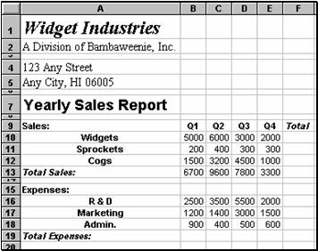
Ø 17317i84r ; 17317i84r ; 17317i84r ; Select B13.
Ø 17317i84r ; 17317i84r ; 17317i84r ; Type =B10+B11+B12. Press Enter.
The cell formula will be displayed in the formula bar, but the answer, 6700, will be in the cell. This is the long way to do things. A quicker way would be to use Autosum
Ø 17317i84r ; 17317i84r ; 17317i84r ; 17317i84r ; Select C13.
Ø 17317i84r ; 17317i84r ; 17317i84r ; 17317i84r ; Type =SUM(C10:C12) Press Enter. SUM is the function. The range within the parentheses, C10:C12, is the parameter.
Ø 17317i84r ; 17317i84r ; 17317i84r ; 17317i84r ;
Select cells D10 through D13, click on ![]() Autosum on
the Standard toolbar.
Autosum on
the Standard toolbar.
Ø 17317i84r ; 17317i84r ; 17317i84r ; Select E10 through E13 click on.
Your screen should look similar to this:
Ø 17317i84r ; 17317i84r ; 17317i84r ; 17317i84r ; Select cell B13.
Ø 17317i84r ; 17317i84r ; 17317i84r ; 17317i84r ; Choose Edit, Copy. A moving border surrounds the cell you are copying.
Ø 17317i84r ; 17317i84r ; 17317i84r ; 17317i84r ; Select cells B19 through E19.
Ø 17317i84r ; 17317i84r ; 17317i84r ; 17317i84r ; Select Edit, Paste.
Ø 17317i84r ; 17317i84r ; 17317i84r ; 17317i84r ; Select cells F10 through F13.
Ø 17317i84r ; 17317i84r ; 17317i84r ; 17317i84r ; Hold down Ctrl and select F16 through F19.
Ø 17317i84r ; 17317i84r ; 17317i84r ; 17317i84r ; Release Ctrl.
Ø 17317i84r ; 17317i84r ; 17317i84r ; 17317i84r ;
Click on![]() . You may see in some cells.
. You may see in some cells.
References Make Formulas More Powerful
With references, you can use data located in different areas in one formula and use one cell's value in several formulas.
Ø 17317i84r ; 17317i84r ; 17317i84r ; 17317i84r ; References identify cells or groups of cells on a sheet.
Ø 17317i84r ; 17317i84r ; 17317i84r ; 17317i84r ; References tell which cells to look in to find the values to be used in a formula.
Ø 17317i84r ; 17317i84r ; 17317i84r ; 17317i84r ; References are based on the column and row headings in a sheet.
Columns are labeled with letters (A through IV, for a total of 256 columns) and rows are labeled with numbers (1 through 16384). This is known as A1 reference style. The reference of the active cell is displayed in the name box at the far left of the formula bar.
Relative References A reference such as A1 tells Excel how to find another cell, starting from the cell containing the formula.
Absolute References A reference such as $A$1 tells Excel how to find a cell based on the exact location of that cell in the sheet. An absolute reference is designated by adding a dollar sign ($) before the column letter and the row number. Using an absolute reference is like giving someone a street address.
Mixed References A reference such as A$1 or $A1 tells Excel how to find another cell by combining a reference of an exact column or row with a relative row or column. A mixed reference is designated by adding a dollar sign ($) before either the column letter or the row number.
Note: Do not use dollar signs to indicate currency within a formula. Use number formatting to determine resulting values.
Applying Number Formats
When creating a new sheet, all cells use the General number format as the default format. When you type numbers in cells formatted as General, Excel assigns the number a built-in format based on what you typed.
Excel assigns a currency format to the cell if you type a $ when entering a value.
Excel includes a variety of number, date and time formats. You can use one of the built-in formats, or you can create your own custom formats. Except for General format, the built-in formats are indicated by symbols that represent how the numbers will look when formatted.
Note: The dollar formats produce a trailing space for positive numbers, so that all amounts align at the decimal point regardless of whether the values are positive or negative.
Use the Number tab in the Cells on Format or the shortcut menu to assign any built-in formats or any custom formats. Custom formats are listed after the built-in formats. We are dealing with dollars in this spreadsheet so we should format the sheet to reflect that.
Ø 17317i84r ; 17317i84r ; 17317i84r ; 17317i84r ; Select column headings B-F.
Ø 17317i84r ; 17317i84r ; 17317i84r ; 17317i84r ;
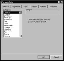
Choose Format, Cells then Number. A dialog box will come up that looks like this:
Ø 17317i84r ; 17317i84r ; 17317i84r ; Select Currency, or scroll down in all and select $#,##0-)-($#,##0). Click on OK. Now you should see a lot of in cells.
Ø 17317i84r ; 17317i84r ; 17317i84r ; Move the cursor between the C and D boundary and double click. All the cells should be in the $15,000 format. If they are not, repeat the first step from above.
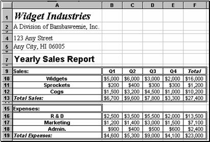
The sheet should look like this:
Adding Borders and Patterns
Excel offers a wide variety of border types and widths, patterns and colors that you can use to create more attractive and effective sheets.
To apply borders, patterns or colors select the cells to be changed and then use these buttons:
![]()
![]()
![]()
Borders button Color button Font Color
The buttons reside on the Formatting toolbar.
You can also choose Cells from Format, or Format Cells from the shortcut menu. Then select the options you want on the Border or Patterns tab.
Note: Adjoining cells appear to share borders. For example, putting a bottom border on one cell produces the same effect as putting a top border on the cell below it. The border does not appear, however, when you print just the cell below. When you print a sheet, borders are printed for a cell only if they are actually applied to that cell.
Ø 17317i84r ; 17317i84r ; 17317i84r ; 17317i84r ; Select the cell or cells to be formatted.
Ø 17317i84r ; 17317i84r ; 17317i84r ; 17317i84r ; From Format, choose Cells then the Border Tab, the shortcut menu, choose Format Cells then Border, or use the border button on the Formatting toolbar.
Ø 17317i84r ; 17317i84r ; 17317i84r ; 17317i84r ; Select your options. To set additional borders using different line styles or colors, select any option under Border and set the style and color for each of the options. For a description of the options, choose Help in the dialog box. Choose OK.
Note: If two cells share a border but each cell assigns a different style to that border, only one border style appears. Excel uses the following order of precedence from least to most dominant to determine which border style to display; no line, dotted line, small dash line, long dash line, light line, medium line, heavy line, double line.
Ø 17317i84r ; 17317i84r ; 17317i84r ; 17317i84r ; Select cell A9. Hold down Ctrl.
Ø 17317i84r ; 17317i84r ; 17317i84r ; 17317i84r ; Select cells B9 through F9.
Ø 17317i84r ; 17317i84r ; 17317i84r ; 17317i84r ; Select cells A10 through A13.
Ø 17317i84r ; 17317i84r ; 17317i84r ; 17317i84r ; Select cells B10 through F13.
Ø 17317i84r ; 17317i84r ; 17317i84r ; 17317i84r ; Choose Format, Cells then the Border Tab.
Ø 17317i84r ; 17317i84r ; 17317i84r ; 17317i84r ; Click on the double border and then on the box to the side of the Outline.
Ø 17317i84r ; 17317i84r ; 17317i84r ; 17317i84r ; Click on the box next to Left and then on the second single border.
Ø 17317i84r ; 17317i84r ; 17317i84r ; 17317i84r ; Click on the box next to Right, Top, and Bottom. Click on OK.
Ø 17317i84r ; 17317i84r ; 17317i84r ; 17317i84r ; Select cells A15 hold Ctrl.
Ø 17317i84r ; 17317i84r ; 17317i84r ; 17317i84r ; Select cells A16 through A19. Then select B16 through F19. Release Ctrl.
Ø 17317i84r ; 17317i84r ; 17317i84r ; 17317i84r ; Choose Format, Cells then Border.
Ø 17317i84r ; 17317i84r ; 17317i84r ; 17317i84r ; Click on the double border and then on the box to the side of the Outline.
Ø 17317i84r ; 17317i84r ; 17317i84r ; 17317i84r ; Click on the box next to Left and then on the second single border.
Ø 17317i84r ; 17317i84r ; 17317i84r ; 17317i84r ; Click on the box next to Right, Top, and Bottom. Click on OK.
To shade cells with patterns
Ø 17317i84r ; 17317i84r ; 17317i84r ; 17317i84r ; Select the cell or cells to be formatted.
Ø 17317i84r ; 17317i84r ; 17317i84r ; 17317i84r ; From Format choose Cells, Patterns; or on the shortcut menu choose Format Cell then Patterns.
Note: To add an outline around a range of cells, select the cells and click the Outline Border tool. To add a border along the bottom edge of cells, select the cells and click the Bottom Border tool. To add shading, select the cells you want to shade and click the Light Shading tool on the Formatting toolbar. To add color to cells, select the cells and click the color tool on the Drawing toolbar until you cycle to the color you want to use.
Ø 17317i84r ; 17317i84r ; 17317i84r ; Select cells A10 through A12 hold down Ctrl and select cells B9 through E12, then A16 through E18.
Ø 17317i84r ; 17317i84r ; 17317i84r ;
Click on ![]() on the Formatting toolbar and choose the medium gray square on the
second row seventh column below the pink square.
on the Formatting toolbar and choose the medium gray square on the
second row seventh column below the pink square.
Ø 17317i84r ; 17317i84r ; 17317i84r ; Select cells A9, hold down Ctrl and select cells A13 and A15 and B13 through E13, then A19 through E19.
Ø 17317i84r ; 17317i84r ; 17317i84r ;
Click on ![]() on the Formatting toolbar and choose the light gray square in the fifth
row last column under the blue square.
on the Formatting toolbar and choose the light gray square in the fifth
row last column under the blue square.
Ø 17317i84r ; 17317i84r ; 17317i84r ; Select cells F9 through F12 hold down Ctrl and select F16 through F18.
Ø 17317i84r ; 17317i84r ; 17317i84r ;
Click on ![]() on the Formatting toolbar and choose the dark gray square in the sixth
row last column under the light gray square.
on the Formatting toolbar and choose the dark gray square in the sixth
row last column under the light gray square.
Ø 17317i84r ; 17317i84r ; 17317i84r ; This will leave cells F13 and F19 white.
Create a New Chart
A chart is a graphic representation of worksheet data. Values from worksheet cells or data points, are displayed as bars, lines, columns, pie slices or other shapes in the chart. Data points are grouped into data series, which are distinguished by different colors or patterns.
Showing data in a chart can make it clearer, more interesting and easier to read. Charts can also help evaluate your data and make comparisons between different worksheet values.
Excel offers 15 basic types of charts to choose from 9 two-dimensional (2-D) chart types and 6 three-dimensional (3D) chart types. Each of the 15 basic charts have between 4 and 10 variations with the total of 102 different kinds of charts. Select from a number of built-in formats for each chart type or add your own custom formatting.
The ChartWizard
The
Chart Wizard![]() is a series of dialog boxes that simplifies creating a
chart. The ChartWizard guides you through the process step by step: you verify your data selection, select a
chart type, and decide whether to add items such as titles and a legend. A sample of the chart you are creating is
displayed so that you can make changes before you finish working in the ChartWizard.
is a series of dialog boxes that simplifies creating a
chart. The ChartWizard guides you through the process step by step: you verify your data selection, select a
chart type, and decide whether to add items such as titles and a legend. A sample of the chart you are creating is
displayed so that you can make changes before you finish working in the ChartWizard.
Embedded Charts and Chart Sheets
Create an embedded chart as an object on a sheet when you want to display a chart along with its associated data.
For example, use embedded charts for reports and documents in which it's best to display a chart within the context of the worksheet data.
Create a chart sheet as a separate sheet in a workbook when you want to display a chart apart from its associated data. You might do this to show overhead projections of your charts as part of a presentation.
Whether you create an embedded chart or a chart sheet, your chart data is automatically linked to the sheet you created it from. When you change the data on your sheet, the chart is updated to reflect these changes.
When you create a chart, you specify the orientation of the data - that is, whether the data series are in sheet rows or sheet columns. Use ChartWizard to change the orientation of the data in an existing chart.
Plotting Nonadjacent Selections
Sometimes the data you are plotting is in rows or columns separated by other data, or by blank rows or columns. You can make nonadjacent selections (sometimes called discontinuous selections) and use them to create a chart.
These nonadjacent selections
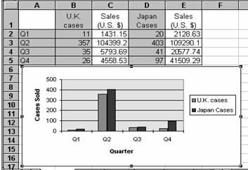
. . . .create a chart showing cases sold, but not dollar sales
Tip: Nonadjacent selections must be a rectangular shape. In cases such as the preceding illustration, in which some cells contain text for series and category names, the blank cell in the upper-left corner of the rectangle must be selected to create the chart correctly.
Ø 17317i84r ; 17317i84r ; 17317i84r ; 17317i84r ; To make nonadjacent selections, begin by selecting cells in the first row or column.
Ø 17317i84r ; 17317i84r ; 17317i84r ; 17317i84r ; To make nonadjacent selections, hold down Ctrl as you make additional selections.
You can also hide rows and columns you do not want to include in your chart, or create an outline and collapse the levels you want to exclude.
When you create a new chart, by default it is a column chart with a legend displayed and some standard formatting applied. You can change these attributes either as you are creating the chart or later, using commands on Format. You can also add items to your chart, using the commands on Insert.
However, if you want most or all of the charts you create to be a type other than column, or to have different formatting, you can change the default format. Changing the default format does not affect existing charts, but all charts you subsequently create will have the new characteristics you specify.
Excel offers two ways to create a chart:
1. 17317i84r ; 17317i84r ; 17317i84r ; 17317i84r ;
The easiest
way to create a chart is through the Default
chart![]() located on the Chart
toolbar. Default chart
creates a chart from data, changes an active chart or an embedded chart to the Default chart format that is specified on the Chart Tab.
located on the Chart
toolbar. Default chart
creates a chart from data, changes an active chart or an embedded chart to the Default chart format that is specified on the Chart Tab.
2. 17317i84r ; 17317i84r ; 17317i84r ; 17317i84r ;
Another way
to create an embedded chart on a sheet is with ChartWizard![]() on the Standard
toolbar. ChartWizard is also available on the Chart toolbar. To create a chart document in a separate window,
use New on File and select Chart.
on the Standard
toolbar. ChartWizard is also available on the Chart toolbar. To create a chart document in a separate window,
use New on File and select Chart.
Using ChartWizard, you can open the embedded chart in its own window to edit or format. Whether the embedded chart is created on a sheet, using ChartWizard or with charting tools, the embedded chart can be saved as a chart document in a separate window. A chart document can also be changed to an embedded chart.
If the Chart toolbar is not displayed:
Ø 17317i84r ; 17317i84r ; 17317i84r ; 17317i84r ;
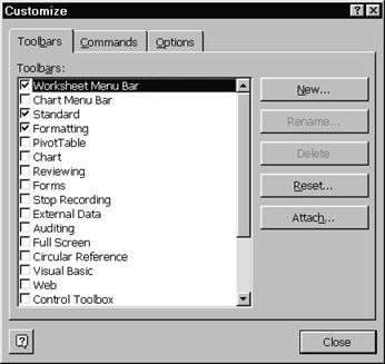
Click on View, Toolbars.
Creating an Embedded Chart on a Worksheet
An embedded chart, is saved as an object on the sheet when you save the workbook.
The embedded chart is always available when the sheet is active, and the chart is printed with the data when you print the sheet. The chart data is still linked to the source data and is automatically updated when the sheet data changes.
Ø 17317i84r ; 17317i84r ; 17317i84r ; 17317i84r ; Select the sheet data you want to display in the chart, and click ChartWizard. The mouse pointer changes to a cross hair with a chart symbol.
Ø 17317i84r ; 17317i84r ; 17317i84r ; 17317i84r ; Select the range of cells A9 through E12. Do not select any empty cells outside the rows and columns.
Ø 17317i84r ; 17317i84r ; 17317i84r ;
Click on ChartWizard![]() . Your cursor
should be a cross hair (
. Your cursor
should be a cross hair (
Ø 17317i84r ; 17317i84r ; 17317i84r ; Place the graph below the data by pointing to the corner of A22 and drag until the rectangle is the desired size and shape.
Ø 17317i84r ; 17317i84r ; 17317i84r ; To plot the chart in a perfect square, hold down Shift while you drag.
Ø 17317i84r ; 17317i84r ; 17317i84r ; To align the chart to the cell grid, hold down Alt while you drag.
Ø 17317i84r ; 17317i84r ; 17317i84r ; Follow the ChartWizard instructions:
Ø 17317i84r ; 17317i84r ; 17317i84r ; The step you are currently on is seen in the top left corner.
Follow each of the steps as follows
Ø 17317i84r ; 17317i84r ; 17317i84r ; Step 1: Next
Ø 17317i84r ; 17317i84r ; 17317i84r ; Step 2: Next
Ø 17317i84r ; 17317i84r ; 17317i84r ; Step 3: Next
Ø 17317i84r ; 17317i84r ; 17317i84r ; Step 4: Next
Ø 17317i84r ; 17317i84r ; 17317i84r ; Step 5: Type Widget Industries Yearly Sales Report in the Title area.
Ø 17317i84r ; 17317i84r ; 17317i84r ; Type Sales in Axes Y
Ø 17317i84r ; 17317i84r ; 17317i84r ; Type Quarter in Axes X
Ø 17317i84r ; 17317i84r ; 17317i84r ; Then click on Finish.
Your graph should look like this:
Excel creates the chart you specified with the ChartWizard. When you use Save or Save As on File to save or name the sheet, the chart is saved with the sheet.
Note: Use ChartWizard to change the data on which the chart is based by selecting the embedded chart on the sheet, click ChartWizard, and select another range of cells on the sheet.
Creating an Embedded Chart on a Worksheet with the Charting Tools:
When you select one of the charting tools on the Chart toolbar, Excel creates an embedded chart on the active sheet. The charting tools correspond to the most commonly used formats for each chart type. If the new chart does not reflect the type and format you want, change by clicking another charting tool.
The following table describes the charting tools on the Chart toolbar:
|
|||||||||||||||||||||||||||||||||||||||||||||||||||||||||||||||||||||||||||||||||
|
|
Area Chart |
Create a simple area chart. |
|
|||||||||||||||||||||||||||||||||||||||||||||||||||||||||||||||||||||||||||||
|
|
Bar Chart |
Create a simple bar chart. |
|
|||||||||||||||||||||||||||||||||||||||||||||||||||||||||||||||||||||||||||||
|
|
Column Chart |
Create a simple column chart |
||||||||||||||||||||||||||||||||||||||||||||||||||||||||||||||||||||||||||||||
|
|
Stacked Column Chart |
Create a stacked column chart |
|
|||||||||||||||||||||||||||||||||||||||||||||||||||||||||||||||||||||||||||||
|
|
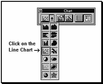
Line Chart |
Create a line chart with data markers |
|
|||||||||||||||||||||||||||||||||||||||||||||||||||||||||||||||||||||||||||||
|
|
Pie Chart |
Create a pie chart with value labels expressed as percentages |
|
|||||||||||||||||||||||||||||||||||||||||||||||||||||||||||||||||||||||||||||
|
|
XY (Scatter) Chart |
Create an XY (scatter) chart with data markers only. |
|
|||||||||||||||||||||||||||||||||||||||||||||||||||||||||||||||||||||||||||||
|
|
Doughnut |
Create a doughnut chart to show more
than one data series, unlike the pie chart. The doughnut chart is widely used in the |
|
|||||||||||||||||||||||||||||||||||||||||||||||||||||||||||||||||||||||||||||
|
|
3-D Area Chart |
Create a 3-D area chart. |
|
|||||||||||||||||||||||||||||||||||||||||||||||||||||||||||||||||||||||||||||
|
|
3-D Bar Chart |
Create a bar chart with 3-D data markers |
|
|||||||||||||||||||||||||||||||||||||||||||||||||||||||||||||||||||||||||||||
|
|
3-D Column Chart |
Create a column chart with 3-D markers |
|
|||||||||||||||||||||||||||||||||||||||||||||||||||||||||||||||||||||||||||||
|
|
3-D Perspective Column Chart |
Create a 3-D column chart with a 3-D plot area. |
|
|||||||||||||||||||||||||||||||||||||||||||||||||||||||||||||||||||||||||||||
|
|
3-D Line Chart |
Create a 3-D line, or ribbon chart. |
|
|||||||||||||||||||||||||||||||||||||||||||||||||||||||||||||||||||||||||||||
|
|
3-D Pie Chart |
Create a 3-D pie chart with value labels expressed as percentages. |
|
|||||||||||||||||||||||||||||||||||||||||||||||||||||||||||||||||||||||||||||
|
|
3-D Surface Chart |
Create a 3-D surface chart. |
|
|||||||||||||||||||||||||||||||||||||||||||||||||||||||||||||||||||||||||||||
|
|
Radar Chart |
Create a radar chart with data markers. |
|
|||||||||||||||||||||||||||||||||||||||||||||||||||||||||||||||||||||||||||||
|
|
Line/Column Chart |
Create a combination chart with a column chart overlaid by a line chart |
|
|||||||||||||||||||||||||||||||||||||||||||||||||||||||||||||||||||||||||||||
|
|
Volume/Hi-Lo-Close Chart |
Create a combination chart with a column chart overlaid by a line chart containing three data series for high, low and closing stock prices. |
|
|||||||||||||||||||||||||||||||||||||||||||||||||||||||||||||||||||||||||||||
|
|
Preferred Chart |
Restores the selected chart to the preferred chart format initially set to format 1 column chart. |
||||||||||||||||||||||||||||||||||||||||||||||||||||||||||||||||||||||||||||||
|
|
ChartWizard |
Use to create an embedded chart or edit the selected chart with the Chart Wizard. |
||||||||||||||||||||||||||||||||||||||||||||||||||||||||||||||||||||||||||||||
|
|
Horizontal Gridlines |
Add or delete major gridlines for the value axis. |
|
||||||||||||||||||||||||||||||||||||||||||||||||||||||||||||||||||||||||||||||
|
|
Legend |
Add or delete a chart legend. |
|
||||||||||||||||||||||||||||||||||||||||||||||||||||||||||||||||||||||||||||||
|
|
Arrow |
Add an arrow to the chart |
|
||||||||||||||||||||||||||||||||||||||||||||||||||||||||||||||||||||||||||||||
|
|
Text Box |
Add an unattached text item. After clicking the tool, type the text you want to appear. |
Ø 17317i84r ; 17317i84r ; 17317i84r ; 17317i84r ; Select the range of sheet cells that contain the data you want to plot, including any sheet column or row labels to be used in the chart. Do not select empty cells outside the rows and columns you want charted. Ø 17317i84r ; 17317i84r ; 17317i84r ; 17317i84r ; Click Line Chart on the Chart type button on the Chart toolbar.
The mouse pointer changes to a cross hair ( Note: To display the charting tool names point to the charting tool Ø 17317i84r ; 17317i84r ; 17317i84r ; 17317i84r ; Move to the next sheet to place the chart. Ø 17317i84r ; 17317i84r ; 17317i84r ; 17317i84r ; Point to A21 and drag until the rectangle is the size and shape you want.
Ø 17317i84r ; 17317i84r ; 17317i84r ; 17317i84r ; To plot the chart in a perfect square, hold down Shift while you drag. Ø 17317i84r ; 17317i84r ; 17317i84r ; 17317i84r ; To align the chart to the cell grid, hold down ALT while you drag. Ø 17317i84r ; 17317i84r ; 17317i84r ; 17317i84r ; Change an existing chart to another chart on the chart toolbar using the Chart type drop down menu. Ø 17317i84r ; 17317i84r ; 17317i84r ; 17317i84r ; Click on an existing chart, when active use the Chart type drop down menu and select another chart. Ø 17317i84r ; 17317i84r ; 17317i84r ; 17317i84r ; The chart will automatically change to the selected chart format. Edit an existing chart You can edit the data in the chart just by editing the data in the sheet. The chart will automatically reflect the changes in your data. You can also edit the parts of the chart such as its title, axes and legends by changing the font, font size and other formatting styles.
Save Your Work Ø 17317i84r ; 17317i84r ; 17317i84r ; 17317i84r ; To save the file, choose File, Save As.
The first time you save a spreadsheet, the Dialog Box will ask for a name for the spreadsheet and the drive and directory in which it will be saved. Save this file on the a: drive. Ø 17317i84r ; 17317i84r ; 17317i84r ; 17317i84r ; Type a:Widget. Click on OK to save the file to disk. Ø 17317i84r ; 17317i84r ; 17317i84r ; 17317i84r ; If it asks you to replace, click on yes. Ø 17317i84r ; 17317i84r ; 17317i84r ; 17317i84r ; You can also click on the directories in the Directories window to choose the destination.
Options saves in different file formats like Lotus 1-2-3, BIFF, Multiplan etc. Always Create Backup File will make a backup file. You can keep people from accessing the spreadsheet by typing in a password in the Protection Password box. Typing a password in Write Reservation Password will give Read access to anyone but Write access to only people with the password. Read-Only Recommended brings up a dialog box to remind users to open a file Read-Only. Ø 17317i84r ; 17317i84r ; 17317i84r ; 17317i84r ;
To Delete a Password, select the
asterisks and press You must know the password to get into the worksheet and delete the password. Once the spreadsheet is saved for the first time, select File, Save to save the most recent changes. If you close Excel and have not saved changes, a dialog box will appear and asks if you would like to save the changes. Sorting DataReorganize data alphabetically and numerically with Ascending Sort and Descending Sort tools on the Standard Utility toolbar or with the Sort command on the Data menu. The Sorting tools on the Standard toolbar is shown below:
When you sort data with the sort tools on the Standard toolbar, you identify the sort key by placing the active cell in the column as the basis of the sort. A sort key identifies which column to sort by. For example, if you want the records sorted by last name, place the active cell in the column containing the last names. Ø 17317i84r ; 17317i84r ; 17317i84r ; 17317i84r ; Open a new spreadsheet: File, New then save as a:names. Move to the next Sheet in your Workbook and type in the following data:
To sort worksheet data with the sort tools Ø 17317i84r ; 17317i84r ; 17317i84r ; 17317i84r ; Select the range you want to sort. Ø 17317i84r ; 17317i84r ; 17317i84r ; 17317i84r ; Place the active cell in the column you want to use as the sort key. Ø 17317i84r ; 17317i84r ; 17317i84r ; 17317i84r ; Select Columns A through C. Or highlight the information you want sorted. Ø 17317i84r ; 17317i84r ; 17317i84r ; 17317i84r ;
To sort the
rows in ascending order, click
the Ascending Sort tool Ø 17317i84r ; 17317i84r ; 17317i84r ; 17317i84r ;
To sort the
rows in descending order, click
the Descending Sort tool Ø 17317i84r ; 17317i84r ; 17317i84r ; 17317i84r ; The rows are sorted in order based on the column that contained the active cell. With Sort, from the Data menu you can specify up to three sort keys and sort by either rows or by columns. The sort key identifies which column to sort by when sorting rows, or which row to sort by when sorting columns. You can refer to any cell in a row or column to identify that row or column as a sort key. When you use more than one sort key, columns or rows with the same entry for the first key are sorted according to the second and third keys. If you have not identified second and third keys, rows or columns with duplicates in the first key are left in the order in which they are found. Ø 17317i84r ; 17317i84r ; 17317i84r ; 17317i84r ; Save your database on the A:\ drive and close this document.
Document InfoAccesari: 2167 Apreciat: Comenteaza documentul:Nu esti inregistratTrebuie sa fii utilizator inregistrat pentru a putea comenta Creaza cont nou A fost util?Daca documentul a fost util si crezi ca meritasa adaugi un link catre el la tine in site in pagina web a site-ului tau.
Copyright © Contact (SCRIGROUP Int. 2025 ) | ||||||||||||||||||||||||||||||||||||||||||||||||||||||||||||||||||||||||||||||