Create Tri command on the Toolbar.

Create Tri command on the Toolbar.

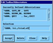
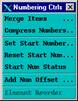
You might find it convenient to establish a command on the Toolbar that turns off the display of the triad at the origin. You do this by accessing the menu controls on the Utility Menu, then choosing to edit the Toolbar.

Enter the command name and command itself as an abbreviation.

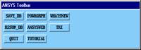
Utility Menu: MenuCtrls Edit Toolbar. Enter tri,/triad,off. Accept. Close.
Execute the triad abbreviation by clicking on the newly created button on the toolbar.

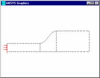
This removed the triad from subsequent displays, and unclutters the display for results plotting.

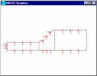
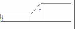
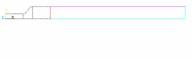
Utility Menu: Plot Lines.

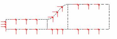
Apply boundary conditions.

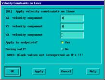
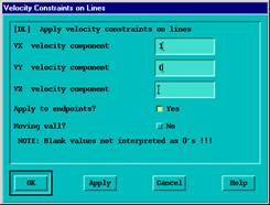
A velocity of 1 inch/second is applied in th 949c29j e X direction (VX) at the inlet, and a zero velocity is applied in the transverse direction at the inlet (VY in the Y direction). Zero velocities in both directions are applied all along the walls, and a zero pressure is applied at the outlet. These boundary conditions are being applied to the lines now so that they do not have to be applied again if re-meshing is required.

Main Menu: Preprocessor > Loads
-Loads-Apply
-Fluid/CFD-Velocity > On Lines.

Pick the inlet line (the vertical line at the far left).

OK in the picker after choosing line.

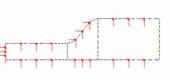
Apply the wall boundary conditions. Choose the lines that make up the walls, then apply zero velocities in the X and Y directions.

Pick the six lines on the top and bottom. OK in the Picker.
Enter 0.0 for VX and VY. OK in dialog box to apply the condition.
Apply the outlet condition. Main Menu: Preprocessor > Loads -Loads-Apply -Fluid/CFD-Pressure DOF On Lines. Pick the outlet line (vertical line on the far right). OK In the Picker.
Enter 0 for the Pressure value. Set endpoints to Yes. OK in the dialog box. Toolbar: SAVE_DB.

At this point, the finite element model is complete and the FLOTRAN menus are accessed to specify the fluid properties along with any other FLOTRAN controls that may be required.

Solution (Laminar Analysis)

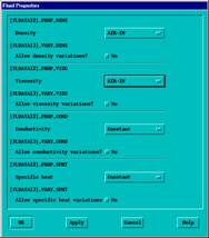
Establish fluid properties.

Fluid properties will be established for air in inches-lb_f-seconds.

Main Menu: Solution FLOTRAN Set Up Fluid Properties. Choose AIR-IN for both density and viscosity. OK in the dialog box shown This produces the next dialog box which confirms the choices - Click OK in it.

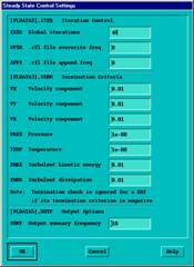
Set execution controls.

Choose the execution control from the FLOTRAN Set Up Menu.

Main Menu: Solution FLOTRAN Set Up Execution Ctrl. Enter 40 Global iterations (Note: 40 global iterations is arbitrary with no guarantee of convergence.). OK to apply and close.

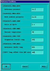
Change reference conditions.

The reference pressure is changed from the default value of 101 KPa to 14.7 psi to maintain a consistent set of units. Likewise, the nominal stagnation and reference temperatures are changed from 293^oK to 530^oR by setting them to 70^oR and adding an offset temperature of 460^oR. See the sections on "Initializing and Varying Properties" and "Using Reference Properties" in the ANSYS CFD FLOTRAN Analysis Guide for additional information on specifying temperatures in absolute or relative scales.

Main Menu: Solution FLOTRAN Set Up Flow Environment Ref Conditions. Change the reference pressure to 14.7 psi (equivalent to 1 atmosphere). Change the nominal temperature to 70oR. Change the temperature offset from absolute 0 to 460oR. OK.
Toolbar: SAVE_DB.

Note: As an option, you might want to zoom-in on the recirculation region (Pan, Zoom, Rotate menu -- click once on the button with the large circle).

Execute FLOTRAN solution.

Main Menu: Solution
Run FLOTRAN.

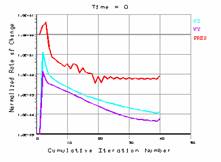
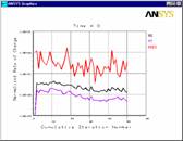
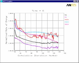
While running the FLOTRAN solution, ANSYS will plot the "Normalized Rate of Change" as a function of the "Cumulative Iteration Number." This is the Graphical Solution Tracker which allows visual monitoring of the solution for convergence.

Close the information window when the solution is done. Leveling off of the pressure monitor implies an oscillating solution.

Postprocessing (Laminar Analysis)

Read in the results for postprocessing.

Enter the general postprocessor and read in the latest set of solution results, and then create a vector plot.

Main Menu: General Postproc
-Read Results-Last set

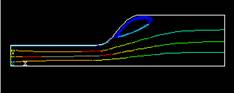
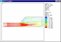
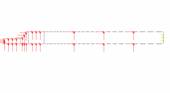
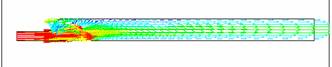
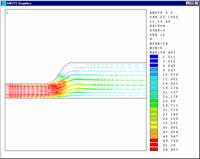
Plot velocity vectors.

Main Menu: General Postproc Plot Results -Vector Plot-Predefined. Vector Plot of Predefined Vectors. OK (without changes).

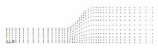
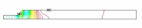
The resulting vector plot shows the recirculation region that occurs in the upper region of the duct.

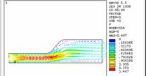
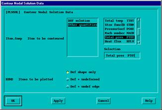
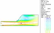
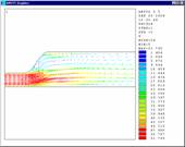
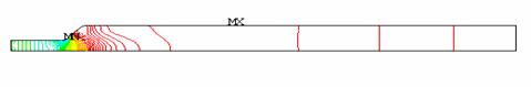
Plot total pressure contours.

Main Menu: General Postproc Plot Result -Contour Plot-Nodal Sol'n. Choose Other quantities in the Contour Nodal Solution Data dialog box. Choose Total Pressure PTOT. OK.

The resulting contour plot shows the total pressures that occur in the duct.

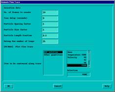
Plot Flow Traces and then Animate them - these show where particles at the inlet or other chosen location travel to

Main Menu: General Postproc Plot Results -Flow Trace-Defi Trace Pt. Pick two or three points around the inlet region and one or two points in the recirculation region (along the upper wall of the transition region). OK (in picking menu). Plot particle traces: General Postproc , Plot Results -Flow Trace- Plot Flow Trac
Utility Menu: PlotCtrls Animate Particle Flow. Choose DOF Solution. Choose VSUM. OK.

Ignore the warning messages about maximum number of loops. ANSYS creates a particle flow path based upon approximations that do not form closed loops.

For Windows NT systems only: the Media Player appears. Make sure the Auto Repeat option is selected before viewing the animation.

For UNIX systems only: make choices in the ANSYS Animation Controller before viewing the animation.

The resulting trace plot shows the path of flow particles through the duct.

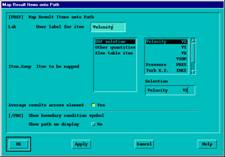
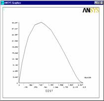
Make a path plot of velocity through the outlet.

Main Menu: General Postproc Path Operations Define Path By Nodes. Pick the lowest and then the highest point of the outlet. OK (in picking menu).
Enter OUTLET for the Path Name. OK.
File Close (for Windows NT/95 systems) or Close (for X11/Motif systems).

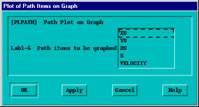
Now specify the velocity in the X direction (VX) to map onto the path.

Main Menu: General Postproc Path Operations Map onto Path.
Enter VELOCITY as label. Choose DOF Solution. Choose Velocity VX. OK.
Main Menu: General Postproc Path Operations -Plot Path Item-On Graph. Choose the label VELOCITY that you previously defined. OK to create path plot.

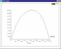
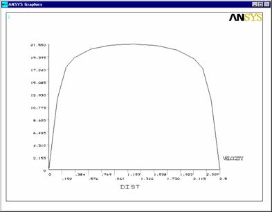
The resulting path plot shows the flow has an almost fully developed laminar profile. The curve looks relatively uniform and has a parabolic shape.

For the next study, you will investigate the effects of increasing the inlet velocity to 50 inches/second.

Solution (Laminar Analysis with Change in Inlet Velocity)

Increase the inlet velocity.

The inlet velocity effects the flow profile. Increasing the inlet velocity by a factor of 50 will increase the Reynolds number accordingly. Return to the apply loads function and change the inlet velocity, then execute the solution.

This is a repeat of step 1.9 with a higher velocity

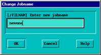
Run the analysis.

This is not a restart of the previous solution. Instead, change the jobname and run the analysis again. Although it is possible to restart a FLOTRAN case from the earlier solution, we choose to start the higher velocity from scratch because occasionally such restarts encounter stall. Stall is when the solution stops progressing towards the correct solution, whereupon the convergence monitors stop decreasing when still at a relatively high value (~1.0e-2). It is due to numerical diffusion, a stabilizing factor in the monotone streamline upwind advection scheme.

Utility Menu: File Change Jobname. Close to exit Solution. Enter "newone" for the new jobname. Change the number of global iterations to 50 OK. Main Menu: Solution Run FLOTRAN.
Once again, the Graphical Solution Tracker is displayed. Close.
Main Menu: General Postproc -Read Results-Last Set. Main Menu: General Postproc Plot Results -Vector Plot-Predefined.
Choose DOF Solution. Choose Velocity V. OK.

Postprocessing (Laminar Analysis Using New Inlet Velocity)

Plot Total Pressure Contours.

This step is a repeat of step 3.3.

Main Menu: General Postproc Plot Results -Contour Plot-Nodal Sol'n. Choose Other quantities. Choose Total Pressure PTOT. OK.

The resulting contour plot shows the total static and dynamic pressures that occur in the duct.

The resulting trace plot shows the path of flow particles through the duct.

5.2 Plot flow traces with new velocity field

Ignore the warning messages about maximum number of loops. ANSYS creates a particle flow path based upon approximations that do not form closed loops.

For Windows NT systems only: the Media Player appears. Make sure the Auto Repeat option is selected before viewing the animation.

For UNIX systems only: make choices in the ANSYS Animation Controller before viewing the animation.

Make a path plot of velocity through the outlet.

Main Menu: General Postproc Path Operations Define Path By Nodes. Pick the lowest and then the highest point of the outlet, just as before. OK (in picking menu). Enter OUTLET for the Path Name. OK.
File Close (for Windows NT/95 systems) or Close (for X11/Motif systems).

The resulting path plot shows the curve has a bias towards one end of the outlet. This indicates that the flow has not yet fully developed. (Note that if your plot appears to be a mirror image of this one, it is because you reversed the order of picking; i.e., you picked the points at the outlet from highest to lowest instead of lowest to highest.)

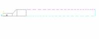
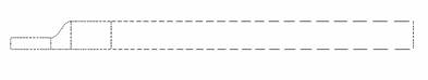
Now in the next study, if the length of the duct's outlet region is increased, the flow may reach a fully developed profile. We will increase the duct length by 30 inches.

Preprocessing (Laminar Analysis with Increase in Duct Length)

The results for the lower viscosity case indicate that the recirculation region has extended well beyond the outlet. To allow the flow to fully develop by the time it reaches the exit, it must be given more room to do so. Many of the steps in the re-analysis outlined below are similar to the previous analysis. Not all menus will be shown over again.

Delete pressure boundary condition.

Main Menu: Preprocessor
Loads
-Loads-Delete
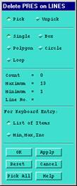
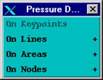
-Fluid/CFD-Pressure DOF
On Lines.

Pick All (in picking menu) to delete all pressure boundary conditions.

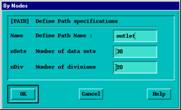
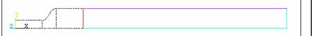
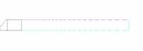
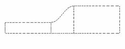
Construct additional outlet region.

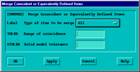
The new rectangle has unique keypoints and lines. These must be merged with their counterparts on the existing areas.
Main Menu: Preprocessor Numbering Controls Merge Items. Choose All for the Type of items to be merged. OK.

A warning message appears stating that an unmeshed line is to merge into a previously meshed line. This is as it should be. Close the message box.

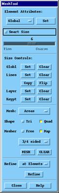
Establish mesh divisions for the new rectangle and mesh.

Main Menu: Preprocessor Mesh Tool. Choose Lines Set. Pick line at new outlet.
OK (in picking menu). Enter 10 for No. of element divisions (as before). Enter -2 for Spacing ratio. Apply.

Repeat this procedure for the upper and lower lines of the rectangle.

Pick lines at the top and bottom of new outlet.
OK (in picking menu). Enter 25 for No. of element divisions. Enter 4 for Spacing ratio. OK.

Flip the line bias on the upper line.

Choose Lines Flip. Pick the upper line.
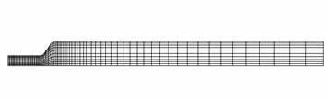
OK (in picking menu). Toolbar: SAVE_DB. Choose Mesh. Pick the outlet area.
OK (in picking menu) to begin mesh. Close the Mesh Tool.

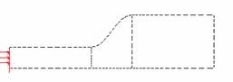
Apply boundary conditions on new region.

Boundary conditions must be applied to the new region. Zero velocities in both directions are applied along the walls, and a zero pressure is applied at the outlet.

Utility Menu: Plot Lines. Main Menu: Preprocessor Loads -Loads-Apply -Fluid/CFD-Velocity On Lines. Pick the new upper and lower walls that don't have boundary conditions.
OK (in picking menu). Enter 0 for VX and VY. OK.

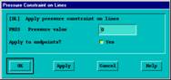
Now apply the pressure boundary condition at the outlet.

Main Menu: Preprocessor Loads -Loads-Apply -Fluid/CFD-Pressure DOF On Lines. Pick the new outlet.
OK (in picking menu). Enter 0 for the Pressure value. Set endpoints to Yes. OK to apply the boundary condition.

Solution (Laminar Analysis Using New Duct Length)

Execute solution.

FLOTRAN will attempt to restart from the previous set of results. If the number of nodes has changed, the program will move the results to jobname.rflo

Execute the new solution, the warning box will appear and disappear by itself.

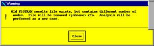
Main Menu: Solution Run FLOTRAN. Close the information window when solution is done.

Postprocessing (Laminar Analysis Using New Duct Length)

Read in the new results and plot velocity vectors.

Main Menu: General Postproc -Read Results-Last Set. Main Menu: General Postproc Plot Results -Vector Plot-Predefined. Choose DOF Solution. Choose Velocity V. OK.

Plot pressure contours.

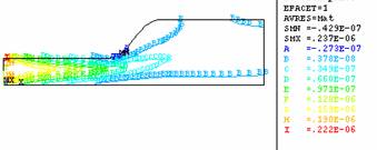
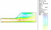
The resulting contour plot shows the static pressures that occur in the duct.

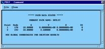
Make a path plot of the velocity through the outlet.

The outlet velocity profile can be examined with a path plot. First, establish a path for the path plot.

Now specify the velocity in the X direction (VX) to map onto the path.

Main Menu: General Postproc Path Operations Map onto Path. Enter "velocity" as the User label. Choose DOF solution. Choose Velocity VX. OK.
Main Menu: General Postproc Path Operations -Plot Path Item-On Graph. Choose the label VELOCITY that you previously defined. OK to create path plot.

The resulting path plot shows that the flow is almost fully developed side of the outlet. Since the velocity has been increased so much, we may be in the turbulent regime. The next step is to check the Reynold's number and activate turbulence if necessary. A consequence of the increased diffusion associated with turbulence is a decrease in the size of the recirculation region.

Calculate Reynolds number.

Calculate Reynolds number in order to determine if the analysis is indeed in the turbulent region (Re > 3000).

Recall that the Reynolds number is determined by the following formula:

Our flow material is AIR, which has the following properties:

r = density = 1.21e-7
V = Velocity = 50
D_h = hydraulic diameter = 2*inlet height = 2
µ = Viscosity= 2.642e-9

Therefore, Re = 4600, which is turbulent.

So the next step is to restart the analysis using the turbulent model.

Solution (Turbulent Analysis)

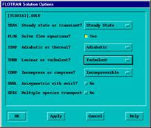
Specify FLOTRAN solution options and execution controls.

Main Menu: Solution FLOTRAN Set Up Solution Options. Choose Turbulent option. OK.

With the increased turbulence resulting from the low viscosity, the nonlinear effects in the problem are more pronounced and more global iterations will be required to achieve a good solution. The number is increased in the Execution Control dialog box.

Rerun the analysis.

Note that this is a restart of the analysis. Restarting an ANSYS/CFD solution requires that the problem domain (specifically, the nodal geometry) is not changed. Since the only changes that were specified were a change the model (from laminar to turbulent) and a change in the number of equilibrium iterations, restarting the analysis is acceptable. Therefore, the solution will pick up where it left off, and 80 global iterations will be executed.

Main Menu: Solution
Run FLOTRAN.

Once again, the Graphical Solution Tracker is displayed.

The preceding postprocessing steps (3.1 - 3.4) can be repeated exactly to show the effects of the higher inlet velocity. These steps are as follows (i.e., repeated steps 3.1 and 3.2): You will see that the recirculation region is smaller due to the increased diffusion resulting from turbulence.

Main Menu: General Postproc -Read Results-Last Set. Main Menu: General Postproc Plot Results -Vector Plot-Predefined. Choose DOF Solution. Choose Velocity V. OK.

Postprocessing (Turbulent Analysis)

Plot Pressure Contours.

This step is a repeat of step 3.3.

Main Menu: General Postproc Plot Results -Contour Plot-Nodal Sol'n. Choose DOF. Choose Pressure PRES. OK.
To obtain a contour plot with more lines, switch to the vector mode and execute on the command line /contour,1,126. Then plot the DOF PRES.

The resulting contour plot shows the total static and dynamic pressures that occur in the duct.

Make a path plot of velocity through the outlet. Follow the steps previously outlined.

Note that with the turbulent model is turned on for the analysis, the flow looks fully developed and the path plot appears to be flatter on the top (instead of parabolic, as in the laminar analyses). Thus the flow is turbulent and the observed results are as expected.

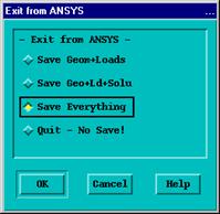
10.3 Exit the ANSYS program.