Contents

Contents

Happy Computers' Telephone Help-Line

More about the help-line

The Happy Computers' Web Site

About this manual

Who is it for and how to use it

What do the icons mean?

Getting Help

The Office Assistant

The Essentials

Starting and closing Excel

The Excel 2000 Screen

The Mouse keeps changing shape

Moving around the spreadsheet

Entering text and numbers

Correcting your mistakes

Undo and Redo - A licence to make mistakes

Saving your Workbook

Closing and Opening your Workbook

Printing your spreadsheet

AutoFill

Selecting parts of a spreadsheet

Inserting and deleting columns and rows

Changing the column widths

Cut, copy and paste

Drag and Drop

Changing the zoom control

Formulas

Using AutoSum

Formulas

Creating a formula

Using percentages

Copying formulas

What are absolute cell references?

Creating and using absolute cell references

Design Principles

The Golden Rules of Good Spreadsheet Design

Range Names

Creating range names

Selecting a named range

Printing a named area

Using range names in formulas

Protection

Protecting your sheet

Putting a password on an Excel Workbook

3-D Workbooks

Working with several sheets

Creating formulas across sheets

Grouping sheets together

Sending Spreadsheets to Word

Pasting information into Word

Functions

Using paste function

If Functions

Count, Counta & CountIf functions

Nested Ifs

Using Excel as a Database

What is a database?

Freeze Panes

Sorting

Auto-Filter

Custom filter

Comments and Text Boxes

Adding Comments to your worksheet

Drawing text boxes

Appendices

What do all the icons do?

What do the error messages mean?

Creating and Using Comments

Glossary

Index

Happy Computers' Telephone Help-Line

Our service does not end when you leave our training centre. For two years from the day of your course you will be able to use, free of charge, our telephone help-line. The aim is to give you the backup to ensure you can confidently do what you covered on your course.

The helpline staff are happy to help out - but please note that the support we can offer is based on the course you attended.
If your question goes beyond the level of the course you attended it is up to the discretion of the Helpline person whether they answer it.  We will always try to point you to another source of help if this is the case.  Please note that the Service Level Agreement cannot be guaranteed in this instance and other calls to the Helpline may take priority over your own."

We want to hear from you. The aim of our courses is to leave delegates confident in using the software. If you have difficulty with any aspect of what you covered on the course, we want to know about it and we want to help you through it.

Your help-line questions also help us. We find out how you use the software, the problems you hit, and sometimes, bugs we don't know about. All this helps to improve our courses and our service. So please keep those calls coming.

You can ring the help-line if you sat on a Happy computers course and for anything covered on that course for up to two years, even if you have changed jobs since doing the course.

It is a guarantee of the quality of our training, so we don't extend it to anyone else in your organisation who has not been trained by us.

(Though ring us if you would like to arrange cover for holidays or sickness)

Access, Excel and web design:  please note that we can't undertake re-design work.  If your database, spreadsheet or web site isn't working because it has been built incorrectly (design faults), we can advise where the problem may lie but we can't do the work for you, I'm afraid.

Outlook: Our training courses use Outlook on an exchange server.  Exchange server can be configured in many different ways,  and you may not be using exchange server at all.  Due to these differences, the menus and other options in Outlook can be very different.  We cannot be responsible for issues that arise due to these differences.

VBA and Javascript:  Sorry, but we won't be able to write code or de-bug yours if it isn't working (unless you are basing your code on an example from our manual). However we may be able to offer you advice on how to change your existing code or point you to VBA resources. Hope that sounds fair.

The help-line hours are 9.30am - 5.00pm. The target speed at which we can resolve your problem depends on which course you have done with us:

Microsoft Excel 2000 Intermediate is a category A course

If you have difficulty getting through please contact Henry Stewart, Managing Director of Happy Computers on 020 7375 7300.

Other sources of help:

Here are some sites that we have found useful for information and problem solving. Please note we are not responsible for anything that appears on these sites and cannot guarantee any of the solutions that you may find on them.

More about the help-line

On 8^th August 2002 Happy Computers Helpline gained TSC Accreditation from the Institute of IT Training, for commitment to high quality support through its service delivery and internal processes. The three main areas assessed were:

Career development, training & assessment for support analysts: clearly defined roles and responsibilities, appropriate technical skills and product knowledge, call handling skills, questioning skills and problem diagnosis, coaching skills

The life cycle of the call - call progression, call escalation, call logging and analysis

The client relationship: service level agreements - promises and undertakings, measurement of satisfaction, call effectiveness and behavioural change.

These are the IITT Assessor's concluding comments:

"Happy Computers Helpline provides a most impressive service to its training client-base. Staffed entirely by 'Helpline Staffers' who have training familiarity with the products they support, they have the ability to provide links to the training courses and continuity to the training process. In the jargon of a traditional helpdesk, the Helpline can demonstrate almost zero tolerance in its compliance with SLA and an almost 100% first time fix rate. The service can frequently boast 'no unresolved calls'.

In conclusion, the Accreditation Consultant reports a highly professional and well managed operation which. conforms with and follows entirely, the ethos of the Institute TSC Accreditation."

Desktop Streaming

We now have the technology to share your screen using t 212o1412c he Internet, thanks to software provided by Desktop Streaming. It is very simple to use and means we can look at your computer screen and help you out immediately over the Internet. It does not require you to have any special software apart from a web browser eg Internet Explorer. The only software that will be downloaded onto your machine is a small chat applet, allowing you to enter into a chat on screen with us if you want to.

It is amazing technology and means that you don't need to worry about emailing a document to us, or trying to explain what you see on your screen! It saves you time and allows us to resolve your query more speedily, improving our customer service to you!

The Happy Computers' Web Site

https://www.happy.co.uk

The Happy Computers web site is dedicated to providing you with information about both the software you use, and the courses we run. You'll find copies of manuals to download and tips on the programs you use, designed to make your work quicker and easier. You'll find up-to-date news about Happy Computers and the team, and you can of course find information on all our courses and book your place on one.

If you have any comments, ideas or just fulsome praise, you can e-mail Colin, our web editor, at: webmaster@happy.co.uk.

Alternatively, write your comments when you do your evaluations on-line at the end of a course at Happy Computers.

If the above means nothing to you, and you are interested in learning more about the World Wide Web and the Internet, Happy Computers run a wide range of courses in Internet software.

About this manual

Who is it for and how to use it

This manual is designed for use with the Microsoft Excel 2000 Intermediate course with Happy Computers.

It is also meant as a back up for when you get back to work in combination with the two year telephone help-line you get free with every Happy Computers course.

It is not meant as a replacement to the full reference manuals that come with Excel 2000

This manual is a step by step guide to the functions taught in the Microsoft Excel 2000 Intermediate course.

You should be able to find the part you're after by looking in the index, and contents and noting that the general course will follow the pattern of the manual.

The step by step parts are in italics. Simply do the things on the left, and read the things on the right for further information

This is what you do This is a description of what is happening

What do the icons mean?

Getting Help

Excel 2000 keeps the screen fairly simple. But don't expect to have to remember the functions. There are several levels of help:

This guide contains all the basic functions of Excel 2000 Use the Table of Contents and the Index to find the functions that you need explained.

The on-screen help function explains commands in detail. It is simple to use

Press F1

Press buttons and scroll bars as required to get more help

For help on a particular part of the screen

Press Shift F1

Click on the area of the screen you wish to know about

To close help

Alt + F4

Or

File menu: Exit (make sure you get the file menu for the help and not for the software)

For more information on using the Office Assistant in Excel 2000 see the next page

Software manuals have improved. Use them as a reference on specific functions, rather than for a general read on how to use the software.

Go to the reference section and look up the thing you want explained.

If you received this manual at a Happy Computers course, we will provide phone support on any functions covered on the course for two years from the date of the course. This is a guarantee of the quality of our training:

Ring: 020 7375 7373 and we will help you with your difficulty. You can do this as many times as you like.

The Office Assistant

Excel 2000 comes with an animated office assistant to help you if you get stuck.

Click on help menu

Click on show office assistant The office assistant will appear (see below)

Type your question into the space provided

Click on search

Click on the blue circle next to the topic you are interested in
Your answer will appear in a new help window

Click on the print icon in the help window

Click on the 'X' at the top right of the help window

Click on the help menu

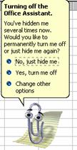
Click on hide office assistant

Click and drag to a new position

Show the office assistant (see previous page)

Right-click on the office assistant A menu will appear

Click on options  A dialog box will appear

Click on the gallery tab at the top of the dialog box

Click on next to move through the assistants

Click OK when you have found the assistant you require

Once you become familiar with the software you may not need office assistant's help so much. If you want to permanently disable it then you can change the options.

Show the office assistant

Right-click on the office assistant A menu will appear

Click on options  A dialog box will appear

Click on the options tab at the top of the dialog box

Un-tick the options you do not require

Click OK

The Essentials

Starting and closing Excel

Click on start 

Click on programs  A new menu will appear to the right

Click on Microsoft Excel

Or if you have a shortcut

Click or double-click on the shortcut icon on the desktop/office toolbar

Click on file

Click on exit

Or

Click on the 'X' at the top right hand corner of Excel

The Excel 2000 Screen

The Mouse keeps changing shape

As you progress through the course you will see that the mouse changes shape all the time, depending on what action you are performing. It's really important that before you start to do anything, you check that your mouse looks correct. Use this page as a reference to remind you what the different mouse shapes mean.

Moving around the spreadsheet

Entering text and numbers

The appearance of a cell changes. Originally you will see a thick border around the cell

But when you enter information the border will become thinner and a cursor will appear

The information you are typing will appear on the formula bar, along with a red cross and green tick

When you have finished typing you must let Excel know by clicking on the green tick or pressing enter, otherwise you will not be allowed out of the cell! Once you have confirmed the green tick and red cross will disappear, and the thick border will return.

Click on the cell you require

Type in the text you require  The border will appear thinner

Press enter or click on the green tick Text will go to the left of the cell

Click on the cell you require

Type in the number you require  The border will appear thinner

Press enter or click on the green tick Numbers will go to the right of the cell

Click on the cell you require

Type the date with forward slashes around it
e.g. 10/3/99

Press enter or click on the green tick

Click on the cell you require

Type the number followed by the percentage sign

Press enter or click on the green tick

Correcting your mistakes

Click on the cell required

Press delete

Click on the cell required

Type the new contents  The original contents will disappear

Double-click on the cell required A cursor will appear inside the cell

Or

Click on the cell required

Press F2 on the keyboard  A cursor will appear inside the cell

Or

Undo and Redo - A licence to make mistakes

Undo allows you to cancel up to 16 of your previous actions if you have made a mistake. If you then decide that you didn't mean to cancel those actions, you can redo up to 16 things that you have undone!

Click on the undo button

Or

Press CTRL & Z

Click on the redo button

Or

Press CTRL & Y

Click on the down arrow next to undo

Find the action(s) you want to undo, scrolling down if necessary

Click the on the action you wish to undo from

Click on the down arrow next to redo

Find the action(s) you want to redo, scrolling down if necessary

Click on the last action you wish to redo

Saving your Workbook

Click on the save icon

Type in a name for your workbook (up to 255 characters)

Change the folder to save in if required

Click on save

Click on the save icon The workbook will be saved in the same place

Using save as will allow you to make a copy of your workbook in a different location or with a different name

Click on file

Click on save as

Type in a new name for the workbook if required

Change the folder if required

Click save

Click on the tools menu

Click on options 

Click on the general tab

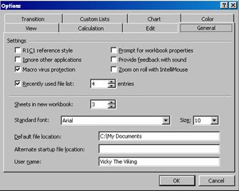Click in the box next to default file location (see below)

Type in the drive and folder you wish to save to, e.g. C:\work

Click OK

Closing and Opening your Workbook

Click on the open icon

Change the folder Excel is looking in if required

Click on the name of the workbook you wish to open

Click on open
or
Double-click the name of the workbook you wish to open

Click on the bottom X at the top right of the screen

or

Click on the file menu

Click on close

Click on the new icon

Or

Click on file

Click on new

Double-click on workbook

Printing your spreadsheet

Click on the print icon

If required, select the area you wish to print

Click on file

Click on print A dialog box will appear (shown below)

If required, click next to selection to print the selected area

If required, type in the pages you wish to print

Type in the number of copies you require

Click OK

If you often print the same section of your worksheet, you can set it as the print area. This means that when you click on print Excel will only print out this area.

Select the area you wish to print

Click on file

Click on print area

Click on set print area  Dots will appear around the selected area

Click on file

Click on print area

Click on clear print area

Click on the print preview icon

AutoFill

AutoFill is a great timesaving feature that allows you to copy text, numbers or formulas in a spreadsheet.

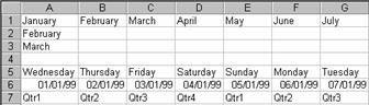
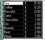
Certain text such as months, days or dates work well with AutoFill. Have a look at the examples below, which were all created using AutoFill

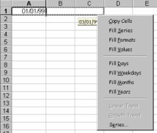
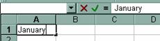
When using AutoFill for dates, for example, you might want the sequence to go from week to week rather than day to day. To achieve this, you must start the sequence off for AutoFill

Type the first date into one cell

Type the second date into an adjoining cell
e.g.

Select both cells

AutoFill as normal

Click on the tools menu

Click on options

Click on the custom lists tab

Select new list on the left hand side

Click in the box underneath list entries

Type your new list into the box, pressing enter after each entry

Click on add when you have finished

Selecting parts of a spreadsheet

Start from the cell at the top left hand corner of the area you wish to select

Make sure that your mouse looks like the big plus sign

Click and drag over the cells you require They will go purple

Click on the column letter you require

Or

Click and drag over the column letters to select several columns

Click on the row number you require

Or

Click and drag over the row number to select several rows

Click on the grey square at the top left corner of the spreadsheet

Select the first area you require

Hold down the control key on the keyboard

Select the second area you require

Inserting and deleting columns and rows

Select the row below where you require a new one

Click on insert

Click on rows  A new row will be inserted above the selection

Or

Select the row below where you require a new one

Press CTRL +

If you select row 6 A new row is inserted above

Select the column to the right of where you require a new one

Click on insert

Click on columns  A new column will be inserted to the left of the selection

Or

Select the column to the right of where you require a new one

Press CTRL -

If you select column B  A new column is inserted to the left

e.g. Inserting six rows

Select six rows below where you require the new rows

Click on insert

Click on rows  Six new rows will be inserted

Or

Select six new rows below where you require the new rows

Press CTRL +

Adjust the number from six to the number of rows you require

Select the rows or columns you wish to delete

Click on edit

Click on delete

Or

Select the columns or rows you wish to delete

Press CTRL -

Changing the column widths

Place your mouse to the right of the column letter you wish to re-size
or
Place your mouse below the row number you wish to re-size

Double-click

Place your mouse to the right of the column you wish to re-size
or
Place your mouse below the row number you wish to re-size

Click and drag to the size you require

Select the columns or rows you wish to re-size

Place your mouse at the right-hand edge of the selected columns
or
Place your mouse underneath the selected rows

Click and drag The columns or rows will all become the same size

De-select the rows

Select the whole of the spreadsheet (see page

Re-size column A to the desired size
And/or
Re-size row 1 to the desired size

Click in the middle of the spreadsheet to deselect

Cut , copy and paste

Drag and Drop

Changing the zoom control

This allows you to stand back from your spreadsheet, so that you can see more of it, or zoom in closer. It does not change the size of the spreadsheet when it is printed

Click on the down arrow next to the zoom control icon

Click on the zoom level you require

Click on the view menu

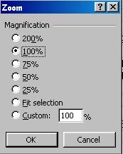
Click on zoom

Click in the circle next to the zoom you require, or type in your own zoom next to custom

Click OK

Formulas

Using AutoSum

AutoSum is a quick and easy way of adding up lists of figures.

Select the figures you wish to add up, the blank cell, and the cell where you require the answer

Click on the AutoSum icon

If you prefer, you do not have to use the AutoSum icon. You can type the formula into the cell instead

Click on the cell where you require the answer (make sure there is a blank row or column between the figures you are adding and the answer)

Type =sum(

Click on the first cell you wish to add up The cell reference will appear

Type a colon

Click on the blank cell at the end of the list The cell reference will appear

Press return or click on the green tick

Formulas

Formula is the term used for calculations in your spreadsheet. The diagrams below show an example formula being entered.

To work out the surplus we need to do a calculation by taking away the expenditure from the salary. You can see this being entered on the left-hand diagram. On the right-hand side you can see what happens once the formula has been completed.

Entering the formula  Completed formula

Formulas always start with the equals sign - that's how Excel knows it's a formula

Cell references are used instead of numbers

A mathematical symbol is used to denote the type of calculation

e.g. Here is the formula from the example above, which found us the surplus (or money left over)

Creating a formula

Once the formula is confirmed the answer will appear in the cell, and the formula will appear on the formula bar.

Calculations are not simply done from left to right. Below is the order in which all calculations are performed.

The acronym for this is BODMAS

Brackets Order Divide Multiply Add Subtract

Using percentages

See page 21

e.g. What is the VAT on a £100

Click on the cell where you require the answer

Type the = sign

Click on the cell containing the percentage, e.g. 17.5% for VAT

Type the asterisk to signify multiplication

Click on the cell containing the number you wish to find a percentage of, e.g. £100

Press enter or click on the green tick

e.g. Finding out what percentage of your salary your rent takes up

Entering the formula Completed formula

Click on the cell you wish to change

Click on the percent icon

Copying formulas

You can copy formula using AutoFill and they will automatically adjust to make sense!

Create your first formula

AutoFill this formula across or down to copy to other columns or rows (See Page )






The formula will not stay the same, but will adjust to make sense!

e.g. This spreadsheet needs totals in row 10, and in column I. To do each formula separately would be time-consuming, so instead, the formula to find the total for January has been copied across to the other months. Likewise, the formula to find the total for rent has been copied down to find the totals for food, social, bills and other.

What are absolute cell references

Using AutoFill to copy formulas is a great way to save time, but you do not always need it to adjust the cell references in the original formula. There are some situations where a cell reference needs to remain constant. Have a look at the example below

In this spreadsheet everyone's salary is due to increase by 10%. The first formula, to find Shing Chen's new salary has been created. We multiply his current salary (cell B4) by the 10% (cell B1)

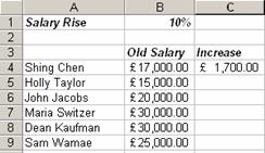
However, everyone's salary is being increased by 10%. If we AutoFill the formula as it is, Excel will adjust the row numbers, and move down from the 10%, and we'll end up with some funny answers.....

If you look at the spreadsheet on the left hand side, you'll see that AutoFill has caused the row numbers to be adjusted. But the formula we need requires cell B1 to remain constant.

So we need to tell Excel to stay at this cell when we AutoFill, and not move down. Excel must absolutely always and forever look at this cell. In other words, we need to make this an absolute cell reference.

Formulas with absolute cell references

Creating and using absolute cell references

Design Principles

The Golden Rules of Good Spreadsheet Design

Always use cell references in formulas and never numbers. If you use numbers:-

Other people using your spreadsheet may not know what the number refers to

If you come back to the spreadsheet a long time after you created it, you may not know what the number refers to

If the number should change, your formula will not update to give the correct answer

It will be difficult to find all the formulas that relate to this number

You will have to change every formula that uses the number, rather than just changing the contents of one cell

Always leave a blank cell between the list of figures and the sum formula. If you do not leave the blank cell, any new information you add may not get included in the formula.

Clean and well-designed spreadsheets calculate downwards and to the right. This makes them easy to follow and avoids circular references.

Circular references occur when a formula loops back on itself. At its most simple, a circular reference can occur when a cell containing a formula is using itself somewhere in the calculation. However, it can also occur when a formula contains a cell reference which happens to contain another formula, and the answer cannot be achieved as both formulas are dependent on the other. Excel then goes round in circles trying to get the answer. You can avoid circular references by ensuring formulae only refer to cells above or to the left.

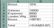
e.g.

In this spreadsheet, a formula in B8 works out the total.
To get the total Excel must add cells B3 to B7.

In cell B6, however, we need a bonus figure. The bonus is the total in B8 multiplied by 10% in B1.
So we cannot get the total in B8 without the bonus, and we cannot get the bonus without the total. Hence we have a circular reference

Mistakes can easily arise through:-

Figures being entered incorrectly

Formulas being typed in incorrectly

New information being typed in that does not get included in existing formulas

So it is essential that you check your spreadsheet with a calculator or by hand.

Range Names

Creating range names

So far we have always referred to cells by their cell reference, e.g. A1, B7. However it can sometimes make more sense to give a cell or cells a name. There are several advantages to doing this

Selecting a named range of cells is a lot quicker and easier

Printing a named range of cells is a lot quicker and easier

Formulas can be clearer and easier to create

Moving around different areas of the spreadsheet can be done more efficiently

Have a look at the example below, which uses range names in a formula

To get the surplus we need to take expenditure away from income. We would normally do this by saying B3-B4. However, if we name these cells as income and expenditure respectfully, then the formula looks clearer and it is easier to see what is happening.

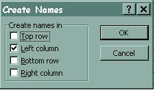
If you have typed the names you would like to use on your spreadsheet already, then you can use them to create range names very quickly!

Click on the insert menu

Click on name

Click on define 

Select the name you would like to delete

Click on delete

Click OK

If you create range names after your formulas, you can change the formulas to use the range name instead of the cell references.

Click on the insert menu

Click on names  A new menu will appear

Click on Apply  A list of your names will appear

Click on the name you wish to apply
or
Hold down the control key and click on several names to apply

Click OK

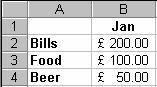
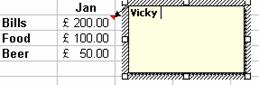
You can name whole columns and rows and then use both the column and the row number as a cell reference. For example in the spreadsheet below you could name column B as Jan, and rows 2,3,4 as bills, food and beer respectively

If you then used the reference Jan Bills (there must be a space between the names), Excel would realise you were referring to cell B2.

Selecting a named range

Click on the drop down arrow next to the name definition box

Click on the range you would like to select or move to

Printing a named area

Click on the drop down arrow next to the name definition box

Click on the range you would like to print

Click on file

Click on print

Choose selection underneath print what

Click OK

Using range names in formulas

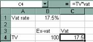
You can type in a range name instead of using the cell reference in a formula.

e.g.

Protection

Protecting your sheet

Once you have set up a spreadsheet, it is all too easy for formulas to get deleted by accident. It's a good idea to protect your spreadsheet to save it from calamity in the future!

Click on the tools menu

Click on protection

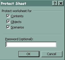
Click on protect sheet

Type in a password if required

Click OK

If you have entered a password, you will be asked to type it in again

You will not be able to change any of the information on your sheet if is all protected

Click on tools

Click on protection

Click on unprotect sheet

You will be asked to enter your password if you set one

When you first create a spreadsheet, all of the cells are formatted as "locked". Any cells that are locked will be protected when you use the protection command. However, if there are cells that you want to be able to change, then you must format them to be "unlocked".

If cells are unlocked then protection will have no effect on them!

Select all of the cells that you want to be able to change
(this is usually all of the cells, except those containing formulas or text labels)

Click on format

Click on cells 

Click on the protection tab

Click on the tick next to locked, so that the box is blank

Click OK

Click on the tools menu

Click on protection

Click on protect sheet 

Enter a password if required

Click OK

If you entered a password, you will be asked to type it again

Now you will be able to change the cells that you unlocked, but everything else will be protected!

Putting a password on an Excel Workbook

If you choose to put a password onto the Workbook, other people will not be able to open it without giving the password

Click on file

Click on save as

Click on Tools

Click on General options.  A dialog box will appear

Type in the password you require next to Password to open

Click OK A dialog box appears

Type password again to confirm

Click OK

3-D Workbooks

Working with several sheets

Excel files are called Workbooks, just like any book they can contain several sheets. To begin with you will have three, but you can add up to 255 sheets or delete the ones that you do not need.

To make your spreadsheet easier to work with! Imagine that you have to store information about your organisation's budget over five years. If you try and put this all onto one sheet, it will become so vast, then it will be almost impossible to navigate through, and find the information you require. But if you set up similar sheets for each year, or even for each month, then it becomes a lot easier to find the information you are looking for.

Click on the sheet tab you require It will become white

Click on the sheet navigation buttons (shown below)

Click on the sheet tab you require It will become white

New sheets are inserted to the right of the selected sheet

Right-click on the sheet tab you require A menu will appear

Click on insert

Click OK

Or

Click on the sheet tab you require

Click on Insert menu

Click on Worksheet

Right-click on the sheet tab you require A menu will appear

Click on delete

Or

Click on the sheet tab you require

Click on edit menu

Click on delete sheet

Click OK

Right-click on the sheet tab you require A menu will appear

Click on rename  The name will be highlighted

Type in the new name

Press enter or click into a cell on the sheet

Creating formulas across sheets

This is useful for obtaining grand totals, on a summary sheet for example. So if you need to add together the contents of the same cell on different sheets, then here is your answer!

Select the cell where the answer will appear

Type =sum(

Click on the first sheet tab to be included

Click on the cell you require

Hold down the shift key on the keyboard

Click on the last sheet tab you require

Click on the green tick or press enter to confirm the formula

In the example below, a grand total of the income in January, February and March was required. Each month had its own sheet, and on each of those sheets the income was held in cell B7. To get the grand total we had to add together the contents of cell B7 on the Jan, Feb and Mar sheets

Grouping sheets together

When sheets are grouped, whatever you do on one sheet will "burn through" to all of the other sheets in the group. It's useful when you are going to have several sheets in a workbook that do virtually the same thing. For instance, you might be creating a budget over several months, and each month has its own sheet. With sheets grouped you can:-

Apply formatting to all of the sheets in the group at once

Create formulas on all of the sheets in the group at once

Click on the first sheet you require

Hold down the shift key

Click on the last sheet you require All the sheets will become white

Click on any sheet that is not in the group

Or

Right-click on any sheet tab

Click on ungroup sheets

The formula will use the same cell references on all of the sheets in the group

Sending Spreadsheets to Word

Pasting information into Word

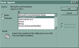
When you perform a straightforward copy and paste (as above) there is no link between the spreadsheet and the word document. If your figures change in Excel, they will not change in Word. If you want to maintain a link between the two you must carry out a paste special.

Make sure that the Excel spreadsheet you are copying from, and the Word document you are copying to, are open

Select the cells you wish to copy

Click on the copy icon

Click on Word on the taskbar

Move your cursor to the position you wish to copy to

Click on the edit menu

Click on paste special

Click next to paste link

Click OK

The spreadsheet and the word document are now linked. If the spreadsheet should change, the table in Word will also change!

Make sure that the spreadsheet containing the chart, and the Word document you are copying it to are both open

Select the chart

Click on the copy icon

Click on Word on the taskbar

Move the cursor to the position you want to copy to

Click on paste icon
or
Click on edit
Click on paste special
Click next to paste link if you require a link

Usually when spreadsheets are copied into Word they behave in the same way as a Word table. However, you may want it to behave like a picture that you can move and re-size easily in Word.

Copy the spreadsheet as usual (see page

Click on Word on the taskbar

Click on edit

Click on paste special

Click on picture, bitmap or picture (enhanced metafile) from the list depending on the type of picture you require

Click OK

It is possible to copy your spreadsheet into Word, and still be able to work on it using Excel's functions.

Copy the spreadsheet as usual (see page

Click on Word on the taskbar

Click on edit

Click on paste special

Click on Microsoft Excel Work Sheet Object

Click OK

Click on the insert spreadsheet icon

Click and drag over the number of columns and rows you require

Functions

Using paste function

There are certain useful calculations that become long-winded if you try and create them with straightforward formulas - such as finding the average of a group of numbers, or rounding numbers up. The paste function in Excel is there to make such calculations quick and easy.

Click on the cell where you require the answer

Type the = sign

Type AVERAGE, MAX or MIN

Type an open bracket

Type in the first cell reference you require (or click on the cell)

Type a colon

Type in the blank cell reference at the end of the list (or you can click on the cell)

Click on the green tick or press enter

e.g.

=Average(A1:A6)

=Max(A1:A6)

=Min(A1:A6)

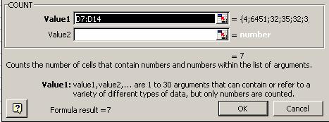
The COUNT function will count the number of cells you select - as long as they contain numbers.

The COUNTA function will count text and numbers but no blanks

Click on the cell where you require the answer

Type the = sign

Type COUNT or COUNTA

Type an open bracket

Type in the first cell reference you require (or click on the cell)

Type a colon

Type in the blank cell reference at the end of the list (or you can click on the cell)

Click on the green tick or press enter

If Functions

An if function asks Excel to consider if something is true or false. If it is true it will return one answer, if it is false it will return a different answer.

e.g.
Can my company afford to buy 10 new computers?
If it is within the budget then "yes", if it is outside the budget, then "no"

Completed if functions Formulas

The structure of an if function always contains the same five elements

Starts with =IF(

The condition followed by a comma

What to do if the condition is true followed by a comma

What to do if the condition is false

Close brackets

For example, the spreadsheet shown above has an if function to work out if 10 computers are affordable. To be affordable they must cost less than the maximum allowable which is £10,000.

To make this IF function easier to understand the condition is underlined, the true part is in bold, and the false part is in italics.

Click on the cell where you require the answer

Type the =IF(

Type in your condition (what you are asking Excel to consider)

Type a comma

Type in what Excel must do if this condition is true

Type a comma

Type in what Excel must do if this condition is false

Close the brackets

Press enter

Select the cell where you require the answer

Click on the paste function icon

If "IF" is not found in the most recently used category, click on logical on the left hand side

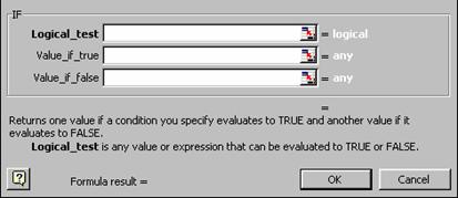
Click on IF on the right hand side

Type your condition next to "Logical Test"

Type what Excel must do if the condition is true next to "Value_if_true"

Type what Excel must do if the condition is false next to "Value_if_false"

Click OK

Count, Counta & CountIf functions

Counts the number of cells that contain numbers

e.g. You want to count how many numbers there are in a list.

The Structure of a count always contains the same three elements

Starts with =COUNT(

The range of cells that Excel is to look at

Close brackets

	=COUNT(C7:C11)

e.g

Counts the number of cells that are not empty. They could contain numbers or text.

e.g. You want to count how many items there are in a list.

The Structure of a count always contains the same three elements

Starts with =COUNTA(

The range of cells that Excel is to look at

Close brackets

	=COUNTA(C7:C11)

e.g

Click on the cell where you require the answer

Type =COUNT(  or =COUNTA(

Highlight the range of cells you are counting from
or
Type in the first cell and the last cell separated by a colon

Press enter or click on the green tick

Click on the cell where you require the answer

Click on the paste function icon

If COUNT or COUNTA is not displayed under the most recently used category, click on "Statistical" on the left hand side"

Click on COUNT or COUNTA You may have to scroll down

Highlight the range of cells that Excel is to count from
or
Type in the first cell and the last cell separated by a colon, next to range

Click OK

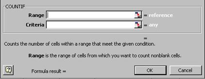
The CountIf function combines the count function and the if function. Use it when you wish to count any cells which match a certain condition.

e.g. This spreadsheet counts how many manufacturers we can afford to buy computers from in cell B14

Completed CountIf function Formulas

The Structure of a count if always contains the same four elements

Starts with =COUNTIF(

The range of cells that Excel is to look at

The criteria which Excel will count from the range

Close brackets

For example, the spreadsheet above counts if manufacturers are affordable. In cells C7 to C11 we are told whether the manufacturer is affordable or not. If they are affordable the text reads "yes."

To make this CountIf function easier to understand the range is in italics and the criteria is underlined.

Click on the cell where you require the answer

Type =COUNTIF(

Highlight the range of cells you are counting from
or
Type in the first cell and the last cell separated by a colon

Type a comma

Type in your criteria

Press enter or click on the green tick

Click on the cell where you require the answer

Click on the paste function icon

If COUNTIF is not displayed under the most recently used category, click on "Statistical" on the left hand side"

Click on COUNTIF You may have to scroll down

Highlight the range of cells that Excel is to count from
or
Type in the first cell and the last cell separated by a colon, next to range

Type in your criteria next to criteria

Click OK

Nested Ifs

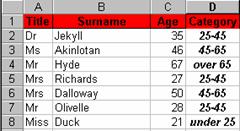
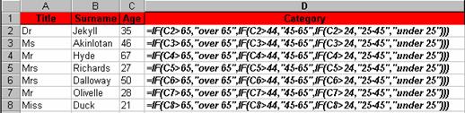
More complicated if functions can require several levels of if. For example the spreadsheet below shows the ages of a group of people. These people are to be put into a category according to their age. So if they are under 25, if they are between 25-45, if they are between 45-65 and if they are over 65 they will be put into a different category.

Completed nested if's

Formulas

Although nested if functions may look nerve wracking, they are just a lot of single if functions strung together (see page ). Before you try them, make sure you have the hang of single if functions. The structure of nested if's is always as follows

Start with =IF(

First condition followed by a comma

What to do if the first condition is true

If the first condition is false then Excel has to move onto the next condition, which will always start with IF(

Second condition followed by a comma

If the second condition is also false Excel moves onto the next condition and this process repeats until you come to the last condition

At the end of the nested if there will be your last condition

What to do if the last condition is true

What to do if the last condition is false

In the example on the previous page, age categories had to be worked out using nested ifs. The Age of all the people was held in column C, starting with C2.

To make this nested IF easier to understand the conditions are in italics, and the true parts are underlined

Type =IF(

Type in your first condition followed by a comma

Type in what Excel must do if the first condition is true, followed by a comma

Type in IF(

Type in your second condition followed by a comma

Type in what Excel must do if the second condition is true followed by a comma

Repeat the process until you come to the last condition

Type in what Excel must do if the last condition is true followed by a comma

Type in what Excel must do if the last condition is false

Close all of the brackets you have opened

Using Excel as a Database

What is a database?

A database is a collection of information with a structure, e.g. a phone book, a card index

Paper databases such as the phone book are much less flexible that a database on computer. There are three main advantages to a database when it is in Excel

It can be sorted into any order
e.g. if the phone book were in Excel you could sort in by the town people live in.
You can also sort on more than one piece of information, e.g. the town people live in, and then alphabetically by their name

Information can be extracted from the whole
e.g. you could extract all the people who live in a certain postal district

You can find information based on anything you know about it
e.g. if the phone book were on computer you would not have to know someone's surname to find them. You could look them up by their first name

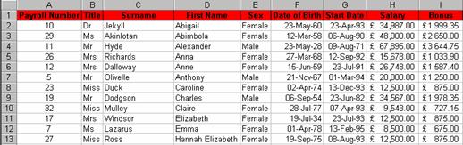
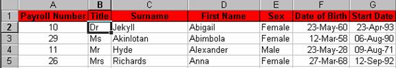
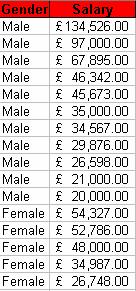
Databases in Excel are usually laid out as shown below

Fields are the types of information you have in your database, e.g. title, surname, firstname, gender, date of birth.
In the example above fields are held in the columns of the spreadsheet

A record is the information for one person or thing
In the example above records are held in the rows of the spreadsheet

Freeze Panes

Often databases in Excel have headings at the top and/or down the side. This makes it a little bit frustrating when you scroll across or down and can no longer see what you are talking about. Freeze panes solves this problem by sticking columns and rows down on the screen where you can always see them.

If you scroll down or across the frozen rows and columns will stay put!

e.g. If you have cell B2 selected:-

Column A is to the left, and row 1 is above the active cell. These will become frozen when you scroll across or down

Sorting

Click into the field you would like to sort by (do not select the column!)

Click on the sort ascending or sort descending icon

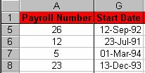
The order in which you choose to sort fields is very important when you sort more than one. The first field you choose is the one which will take precedence over the other sort orders.

e.g.

Department first, and then Surname Gender first and then salary

Select any cell inside the database

Click on data

Click on sort

Click on the down arrow next to the top rectangle and choose the field you would like to sort by first

Click on the down arrow next to the second rectangle and choose the field you would like to sort second

If required, click on the down arrow next to the third rectangle and choose the field you would like to sort third

Click OK

Auto-Filter

You can use AutoFilter to extract or find information in your database

Click on data

Click on filter

Click on AutoFilter 

When AutoFilter is turned on down arrows will appear next to field names

Turn AutoFilter on

Click on the down arrow next to the field you would like to filter

Click on the criteria you would like to see

Turn AutoFilter on

Click on the down arrow next to the field you filtered

Click on All

Or

Click on data

Click on filter

Click on show all

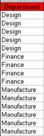
e.g. All the males in the finance department

Click on data

Click on AutoFilter

Click on the down arrow next to the first field you wish to filter

Click on the down arrow next to the second field you wish to filter

Custom filter

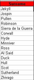
Making comparisons between numbers, e.g. greater than, less than

Specifying parts of text, e.g. starts with "S", ends with "son"

Finding dates before or after, e.g. before 1999

Turn AutoFilter on

Click on the down arrow next to the field you wish to filter

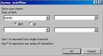
Click on custom

Click on the down arrow next to the equals

Click on the comparison you would like to make

Type in your criteria in the blank rectangle next to the comparison

Click OK

Turn AutoFilter on

Click on the down arrow next to the field you wish to filter

Click on custom

Choose "is greater than or equal to" as your first comparison

Type in the earlier date or the smallest number in the box to the right

Make sure that "and" is selected in the middle

Choose "is less than or equal to" as your second comparison

Type in the later date or the largest number in the box to the right

Click OK

Comments and Text Boxes

Adding Comments to your worksheet

Adding comments to your worksheet helps you understand what you have done. They will be hidden until you choose to see them.

Select the cell that will contain the note

Click on insert

Click on comment A comment box appears (see below)

Type in your comment

Click outside the comment box  A red triangle appears in the cell

Hover your mouse over the red triangle  Comment will appear

Right-click on the cell with the comment

Click on delete comment

Right-click on the cell containing the comment

Click on edit comment  Comment box will appear with a cursor for you to type

Right-click on the cell containing the comment

Click on show comment/hide comment

Click on file

Click on page set-up

Click on sheet tab

Click on down arrow next to comments section

Click on At end of sheet

Click OK

Drawing text boxes

Text boxes are similar to comments, except they are always visible on your worksheet

Make sure the drawing toolbar is displayed (see below)

Click on the text box icon

Click and drag the shape of a box onto your spreadsheet

Click inside the box and type your note

Click outside the box when you are finished

Select the text box to move  Diagonal lines will appear around the edge

Click on the diagonal lines  Dots will appear around the edge

Hover the mouse over the dots until it changes to a four-headed arrow

Click and drag the text box to a new location

Select the text box to re-size  White boxes will appear around the edge

Hover the mouse over a white box till it changes to a double-arrow

Click and drag to re-size the text box

Select the text box to delete  Diagonal lines will appear around the edge

Click on the diagonal lines  Dots will appear around the edge

Press delete on the keyboard

Appendices

What do all the icons do?

What do the error messages mean?

When something goes wrong with a formula Excel produces messages that attempt to describe what the problem is:-

Creating and Using Comments

When more than one person use the same workbook, some users may wish to affix notes to some of the data and notify other users of why they had made certain changes. You could also wish to put a help note on a particular cell such as which key strokes to press to enter the date automatically.

A cell with a comment is marked by a red triangle in the top left hand corner and you can access the note by hovering the mouse over the triangle.

Select the cell to which you wish to attach a comment

Click on Insert

Click on Comment

Type your comment in the box

Click outside the box when your comment is complete

Select the cell which contains the comment you wish to change

Click Insert

Click Edit Comment

Make your changes

Click outside the comment box

The reader can review all comments that have been attached.

Click on View

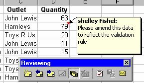
Click on Comments

The comments and the Reviewing Toolbar appear

The first comment is shown

Click next comment on the reviewing toolbar to view each comment in sequence

Click Previous comment to see comments in reverse order.

There are times when you may not want the comments or their indicators to be visible in the workbook.

To Hide Comments:

Click on Tools

Click on Options

Select the View Tab

Under Comments select either NONE - does not display the comment indicator and hides comments even when you rest the pointer over the cell.

OR

Comment Indicator Only - Displays indicators but comments only appear when you point at the comment cell.

OR

Comments and Indicator - Displays the comments and indicators regardless of where the pointer is.

Click OK

To see hidden comments again:

Click View

Click Comments

You can print comments when you print the worksheets:

Click the worksheet that contains the comments

Click on File

Click Page Setup

Select the Sheet Tab

From the Comments drop down list select

At End of Sheet - to have comments print at the end of the worksheet

As Displayed on Sheet - to have comments print where they are shown( make sure View, Comments was selected first)

Click Print

Select the appropriate options from the print dialogue box

Click OK

Select the cell which contains the comment

Click Edit

Click Clear

Click Comments

Glossary

If you want to copy a formula to another cell, but you want to prevent Excel from adjusting the cell references, make the cell references "absolute". Absolute cell references are indicated by a dollar sign ($).

The cell border of the active cell is darker than the other cells, and indicates the cell you are currently working on

This feature is useful when you need to enter a series of numbers, dates or formulas

This will automatically format your table, for example adding heavy lines to form a box around the date

This feature allows you to select the cell range containing the values that you wish to add together. It then adds those figures up.

This is the basic building block of the Excel worksheet. A cell if formed by the intersection of the row and column gridlines. Each cell is identified by the letter of the column and the number of the row. E.g. B7

A group of cells that are next to each other.

These are the co-ordinates of the cell in the worksheet, e.g. B7

This is a sheet in a workbook containing a chart. The chart sheet is updated when the worksheet data is changed.

This is a solid black square in the right hand corner of the active cell border. Using your mouse, grab the black square and drag it across to AutoFill your cells.

Formulas are the basis of Excel. Formulas will do all the calculations that will normally be done by a calculator. You can use formulas to do simple calculations such as additions, subtractions, multiplication, division as well as statistical, financial and scientific calculations.

This is the bar at the top of the Excel screen. It is used to enter and edit formulas and values. It also displays the formulas in a particular cell.

These are the lines that you see in your spreadsheet. You can choose to print them using the tools menu, then the options dialog box.

This is the text which usually appears next to the figures in a spreadsheet, and identifies what the figures mean.

A legend (also known as a key) is used in charts and graphs. Excel actually creates legends from the labels on the worksheet. The legends can be customised with borders, patterns and different fonts.

In a formula there can be a combination of relative and absolute cell references. A mixed reference can look like this $A1 or A$1. $A1 refers to column A regardless of the position of the cell containing the formula.

This allows you to enter commonly used calculations quickly, such as finding the average, maximum or minimum of a group of numbers.

Relative cell references are used in formulas where you do not wish the reference to remain constant as the formula is AutoFilled. Relative cell references do not contain the $ found in absolute cell references.

It is possible to insert, delete, rename, move and copy sheets in Excel. The sheet can be a worksheet, chart sheet, module sheet or dialogue sheet. A worksheet is the most often used.

This is also called a spreadsheet. The worksheet is the primary document used in Excel. A worksheet is made up of cells in columns and rows and is always part of a workbook.

Index

Absolute cell references  48

creating  49

Adding 41

Auto Filter  90

AutoFill  29

AutoSum 41

Changing

Contents of a cell  22

Charts

Copying into Word  71

Closing

Excel 16

workbooks  26

Columns

changing the width  35

Deleting  34

inserting  33

selecting  31

Comments  94

Creating  100

Editing 100

Hiding 100

Printing  100

Removing  103

Reviewing  100

Constants  48

Copying

Cells 36

Drag and drop  38

formulas  47

Into Word  70

Sheets 66

Correcting

mistakes  22

CountIf 81

Cut 36

Dates

Entering  21

Default folder  25

Deleting

Contents of a cell  22

Range Names  55

rows and columns  34

Sheets 66

Design 51

DIV/O! 99

Drag and Drop  38

Editing

Contents of a cell  22

Entering  20

Dates 21

Numbers 20

Percentages  21

Text 20

Error Messages  99

Exiting

Excel 16

F4 48

Formatting Toolbar  98

Formulas

Average, Max, Min  75

copying 47

Count 75

creating  43

definition  42

Over different sheets  67

Freeze panes  87

Golden Rules  51

Grouping Sheets  68

Help 12

Icons 97

If function  76

Inserting

rows and columns  33

Keyboard

Moving around  19

selecting  32

Mistakes  22

Mouse Shapes  18

Moving 19

Drag and drop  38

Moving Sheets  66

N/A! 99

NAME? 99

Naming

Ranges 54

Sheets 66

New

rows and columns  33

workbooks  26

NULL! 99

NUM! 99

Office Assistant  13

Opening

Workbooks  26

Page breaks  28

Passwords  61, 63

Paste 36

Paste function  74

Percentages  45

Entering  21

Print Preview  28

Printing

spreadsheets  27

Protection  61, 63

Range Names  54

Deleting  55

Redo 23

REF! 99

Replacing

Contents of a cell  22

Row

inserting  33

Rows

Deleting  34

selecting  31

Rules 51

Saving 24

Default folder  25

Screen 17

Security  61, 63

Selecting  31

Sheets 65

Copying 66

Deleting  66

Grouping  68

Moving 66

Re-naming  66

Sorting 88

Spreadsheet

selecting  31

Spreadsheet Design  51

Standard Toolbar  97

Starting

Excel 16

Text

entering  20

Text boxes  95

Toolbars

Formatting  98

Standard  97

Typing in  20

Undo 23

VALUE! 99

Width

of columns  35

Word 70

Zoom control  39