Simulation examples
In this section we look at some examples to illustrate the new approach. In the first subsection we are going to compare for different penalty coefficients the pseudo-log-optimal portfolios with each other. Then we look at the behaviour of the pseudo-log-approach compared to the log-optimal approach. We will also include two kinds of transaction costs to approach to the reality, i.e. we derived the methods in a market with no transaction costs, but consider the resulting strategies in situations close to the reality.
We consider a market with one risky asset and one risk free asset.
Let ![]() be given. We choose
be given. We choose ![]() and the initial capital
and the initial capital![]() .
.
The log-optimal portfolio is given by

We choose

From Chapter 2 and 3 we have the following equations, which we need for the simulation:
The log-optimal wealth process is given by
![]()
The price processes are
![]()
![]()
The optimal trading strategy from the new approach is given by
![]()
where


and
![]()
Setting in the coefficients from above in the optimal controls and get

From section 3.3 we had for the initial optimal trading strategies
![]() (*)
(*)
![]()
With the definition of the optimal trading strategy we can give formulation for the pseudo-log optimal wealth process
![]()
The trading takes place during the time interval [0,10]. We only consider the trading strategy of the risky asset, because it does not matter how much the trading strategy of the risk free asset fluctuates.
Now we have stated all equation we need to simulate the log-optimal and pseudo-log-optimal trading strategies and wealth processes.
We simulate and programme this in Matlab.
3.4.1 Comparison of the penalty coefficients
In Remark 11 i) we did mention the meaning of the penalty coefficients. Their changes influence the optimal controls and so the optimal trading strategies. Here we visualise the trading strategies for five different constant penalty coefficients.
Let the penalty coefficients be given as
![]()
For one
price realization the trading strategies corresponding to these penalty
coefficients are given in the picture below, where the blue line corresponds to
the trading strategy with![]() , the red line to
, the red line to ![]() and so on (See above).
and so on (See above).
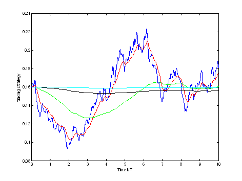
One can see
that if the penalty coefficients are getting bigger, then
the trading strategies processes are getting nicer, i.e. the changes are
getting smaller. For the biggest penalty coefficient and the smallest, the
difference is huge. The trading strategy corresponding to ![]() fluctuates much, where
the trading strategy corresponding to
fluctuates much, where
the trading strategy corresponding to ![]() is almost constant.
is almost constant.
This is a nice difference if we would calculate the transaction costs.
Remark 13: (important for 3.4.2 the third example)
The trading strategy corresponding to the biggest penalty coefficient seems to be constant, but it is not. It still changes in every step a little bit, so that for fixed transaction costs we still would loose the whole money as in the log-optimal case (See 2.5). And this is true for all penalty coefficients, i.e. we handle almost as much as in the log-optimal case. The only difference is that the total transaction value is smaller in the new approach.
The corresponding wealth processes are given by
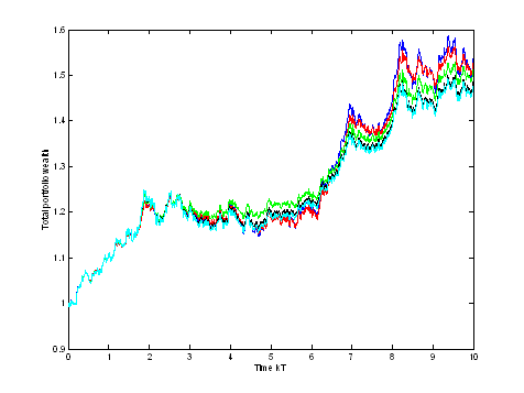
At the beginning all five wealth processes are the same. The difference between the processes is visible at the end, which is not big. Here we see that the wealth process corresponding to the smallest penalty coefficient is the best at the end, where the one with the biggest penalty coefficient is the worst.
But let us consider another price realization. The penalty coefficient and the colours allocation are the same. Then we have for the trading strategies
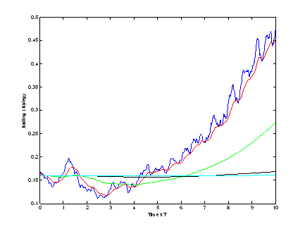
Again we have the same distributions. The one with the biggest penalty coefficients fluctuates at most and the one with the smallest at less. But now the total wealth processes are given by
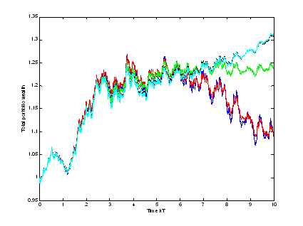
Now one can see that two wealth processes, which belong to the trading strategies with the smallest fluctuations, are the best.
Till now we had once that the total wealth with the biggest penalty was the best, and once the one with the smallest. Next we want to see how they act in average. For 100 different price realizations we get for the five total wealth
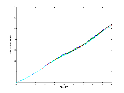
In average the differences between the processes are very small. To see this exactly we have enlarged the time interval [9,10]
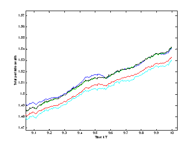
Summary: We did see that for different penalty coefficients we get different trading strategy processes and in average almost the same wealth processes. For big penalty coefficients we get a very nice form of the trading strategy and in average the same wealth process as for a small penalty coefficient. It is a wonderful result, if we would care about the trading strategy and its behaviour as in the case where we have transaction costs. Then we would of course favour the trading strategy with the nicest process.
3.4.2 Pseudo-log-optimal and log-optimal approach
In this subsection we will see the advantages and disadvantages of the pseudo-log-optimal portfolio in comparison with the log-optimal portfolio. We give some examples with including of some kind of transaction costs to bring the whole setup closer to the reality.
Examples:
We illustrate
the pseudo-log-optimal portfolios for two different values of b, i.e. ![]() and
and![]() .
.
In all
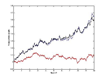
following pictures we have that red line belongs to the log-optimal case, the
blue line to the pseudo log-optimal with![]() and the black line to
and the black line to![]() .
.
1) In this first example we show the trading strategies and the total wealth developments for one price realization. We do not consider any kind of transaction costs, i.e. we are in the same market where we derived the portfolios.
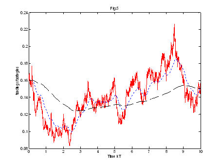
Fig.3 shows
us the trading of stock for the log-optimal and the pseudo-log optimal
portfolios. One can see that the trading strategy![]() of the stock for the log-optimal portfolio (red line)
fluctuates at most, where for
of the stock for the log-optimal portfolio (red line)
fluctuates at most, where for ![]() the trading strategy
the trading strategy ![]() (black line) has very small changes. The trading strategy
corresponding to
(black line) has very small changes. The trading strategy
corresponding to ![]() (blue line) has the
same trend as the log-optimal one, but do not fluctuate so rapidly. (The
difference between the two pseudo-log-optimal trading strategies will be
explained in the next subsection)
(blue line) has the
same trend as the log-optimal one, but do not fluctuate so rapidly. (The
difference between the two pseudo-log-optimal trading strategies will be
explained in the next subsection)
Let us look at the total portfolio wealth corresponding to these trading strategies.
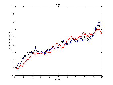
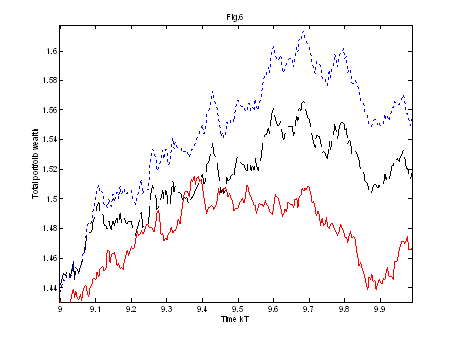
Fig.6 shows us the three total portfolios wealth. In Fig.7 the end period [9,10] is enlarged.
One can see that they have almost the same development. Both pseudo-log-optimal total portfolios wealth are a little bit better than the log-optimal one at the end.
That means
for this stock price realization we have that the final wealth of the
log-optimal portfolio is little bit worse than the pseudo-log-optimal, but the
trading strategies are totally different, i.e. the trading strategy of the
log-optimal portfolio fluctuates a lot, so we would pay a great amount of
transactions costs (if we would consider them), but the trading strategy of the
pseudo-log optimal portfolio (especially for ![]() ) doesn't fluctuate so much, and so the transaction costs would
be smaller as in the log-optimal case.
) doesn't fluctuate so much, and so the transaction costs would
be smaller as in the log-optimal case.
Summary: With the new approach we reach a better result for the end wealth for one prize realization, where the corresponding trading strategies do not fluctuate like the log-optimal one.
Let us now have another price realization. Then the trading strategies look like follows:
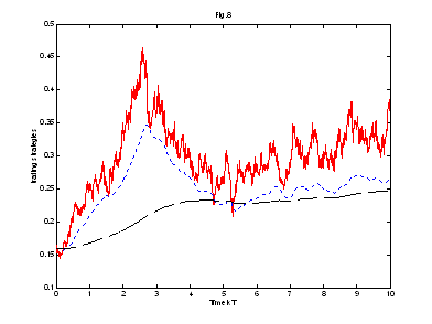
where we have the same notations as before. Again the trading strategies of the log-optimal portfolio fluctuates more than the other two's. But for this realization of the stock price we have the following total portfolio wealth development:
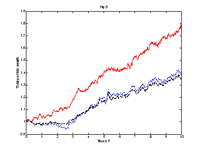
Now one can see that the log-optimal total portfolio wealth is much bigger than the pseudo-log-optimal total wealth. One should not wonder why once the log-optimal is better and once worst. We did maximise the expectation to get the log-optimal or pseudo-log-optimal strategies. But it means not, that if we simulate it that it is not random.
To see how both behave in expectation (or in average), we have to take for several price realizations the average, i.e. for n price realizations we have for the log-optimal wealth process for each k
![]()
and for pseudo-log-optimal
![]()
where ![]() denotes the log-optimal portfolio wealth in step k for the
j-th price realization and
denotes the log-optimal portfolio wealth in step k for the
j-th price realization and ![]() the pseudo-log-optimal wealth in step k for the j-th price
realization. For n=150 different price realizations we get the following wealth
processes:
the pseudo-log-optimal wealth in step k for the j-th price
realization. For n=150 different price realizations we get the following wealth
processes:
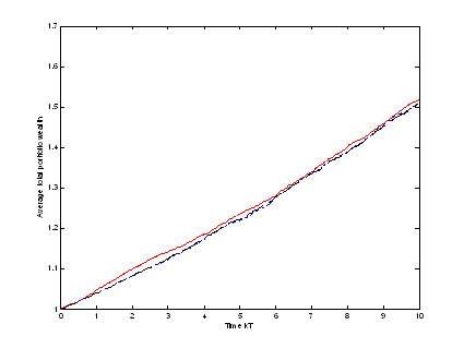
Now one can see that the log-optimal wealth process is always above the pseudo-log-optimal. But this is clear, since we have for all k
![]()
Up to now we have seen that the pseudo-log-optimal wealth process can be better for some price realizations than the log-optimal, but in average it is not. The difference between the two processes, as a drawback for the pseudo-case, can be big (as seen Fig. 9), but in average it is really small. Because of such nice results the new method is great, since for almost the same end wealth we did reach to have trading strategies with a nice moving, without fluctuating much.
2) In this example we are going to consider one kind of transaction costs. Then we can see the advantage of the new method. There are two cases we will deal with. The first is if we calculate the transaction costs without subtracting them. The other is to subtract them directly step for step from the wealth in the corresponding step.
Remark 16:
One should note that we did derive us the log-optimal and the pseudo log-optimal portfolio in a market with no transaction costs. But now we want to see how they act in situations, which are closer to the reality. And so we have to consider transaction costs.
We still assume
there is no transaction cost for the bank account. The transaction cost that
would have accumulated at time ![]() for the log-optimal
for the log-optimal![]() and the pseudo-log-optimal
and the pseudo-log-optimal![]() , are given by:
, are given by:

That means at every step we take 1% of the total transaction value of buying or selling shares of the stock.
Remark 17:
Note that we still consider the forward induction case, i.e. we go from one step to the other. Because of that we have such a transaction costs equation, which accumulate form one step to the other.
To see that we really take 1% of the total transaction values in both transaction costs equations for each step do as follows:
For the second equation this is clear, since at time (k+1)T we posses the following amount of money in stock before rebalancing
![]()
and after rebalancing
![]() .
.
That means that the total transaction value in stock is
![]()
Taking one
percent of that and get the transaction cost equation for![]() .
.
To see that the transaction cost structure for the log-optimal case is also just the 1% of the total transaction value we reformulate the equation:

After this examination we have still to take us the 1% of the initial total transaction value, i.e.

Now we can calculate the transaction costs for the whole period.
i) Here we concentrate us on the first case, where we only calculate the transaction costs. We take the same price realization as in the first picture, where the pseudo-log-optimal was better than the log-optimal.
The total
wealth X(10) and the transaction cost ![]() at the end of trading
period are:
at the end of trading
period are:
Log-optimal
portfolio: ![]()
Pseudo-log-optimal:
![]()
![]()
![]() :
: ![]()
The final wealth of the pseudo log-optimal portfolio is better (as seen in figure 4 and 5).
The transaction costs compares are very amazing:
![]() :
: ![]()
![]() :
: ![]()
i.e. for ![]() we have that
the transaction costs for the log-optimal are 11 times higher than in the
pseudo-log-optimal case, and for
we have that
the transaction costs for the log-optimal are 11 times higher than in the
pseudo-log-optimal case, and for ![]() 25 times higher. This
is the consequence from the nice movements of the new trading strategies.
25 times higher. This
is the consequence from the nice movements of the new trading strategies.
That means for a bigger final wealth, we get with the pseudo-log-optimal portfolio also 11 times or 25 times smaller transaction costs. This is a very nice example and a confirmation for the new approach.
Let us have the realization of the stock price, where the log-optimal is much better than the pseudo-log-optimal. Then we have
Log-optimal portfolio: ![]()
Pseudo-log-optimal:
![]()
![]()
![]() :
: ![]()
![]() :
: ![]()
![]() :
: ![]()
The transaction costs are still much higher in the log-optimal portfolio, but now the final wealth is also higher. This is a nice example where we have a reduction of the transaction costs, but as a payoff a smaller profit.
Because of the movements of the trading strategies, we have always a reduction of the transaction costs. But this will only make a difference between the end wealth, if they are almost the same.
Remark 17:
In this example we did calculate the transaction costs, but we do nothing with them. First we just wanted to see the big difference of the trading strategies respectively the resulting transaction costs. Second, one can subtract the accumulated transaction costs from the final wealth, and simulate so a market with transaction costs. Of course this is fake, because one has to pay transaction costs at each step one handle. This will be done in the next example.
ii) Let us be some more realistic and subtract the transaction costs directly in each step. Then for one price realization we get Fig.., where we have that the pseudo-log-optimal is much better than the log-optimal.
For another price realization we get
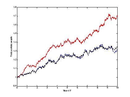
Here one can see that the log-optimal is much better. The reduction of the transaction costs does not pay off for this price realization. Again we have to argument that the randomness is not excluded, we just did maximise the expectation.
Of course the next aim is to see how they act in average. Fig. shows for 100 different price realizations the average of the two methods.
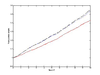
Here we can see a wonderful result for the new approach. The pseudo-log-optimal total wealth is in average clear better than the log-optimal. In average the reduction of the transaction costs pay off.
3) Here we will consider fixed transaction costs. We know from Chapter 2 that the log-optimal wealth process act terrible by including this kind of transaction costs. This is also the case in the new approach, because we handle at any time instant independent of the penalty coefficients (See Remark 15) as in the log-optimal case. Because of that it does not matter that the total transaction value is smaller as in the log-optimal case, since we consider fixed transaction costs.
For one price realization we get for the wealth process (for fixed transaction costs of 0.0004)
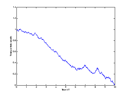
We loose the whole money trading with the pseudo-log-optimal strategy.
|