TASK 3.1

This example will build on the name counting-code you created in exercise 1.6.2. This exercise will lead on to an investigation of some of the characteristics of Excel objects and show how the use of worksheet controls (i.e. buttons, listboxes, checkboxes etc) both improves the efficiency of our applications as well as to making them more user-friendly.

This first task is quite simple. You have a list of names, together with their earni 22122m128w ngs for various jobs. Each name can be repeated, since each row relates to a single job. The data might look something like this.

The task is to write a VBA macro which

asks for a name

searches through the list, adding up the totals for that name

highlights the relevant rows and reports the sum

Here is some code for this purpose:

Note the weaknesses of this approach - it is essential for the name to be typed in exactly as it appears in the spreadsheet if this is to work. We will see shortly how a worksheet control will help here.

TASK 3.2 : Using Excel Worksheet Controls

When customising Excel to carry out a particular task, one of the most important areas is that of data entry and manipulation. A typical application for Excel involves the representation of a 'model', specified by worksheet formulae, which is to be analysed. The 'output' may be represented graphically (or numerically) and the input (i.e. the values of certain key parameters in the model) is supplied by the user.

This input can be assisted by the use of worksheet controls. To simply provide an empty cell into which the user would enter the numerical value required for a given parameter can lead to problems if an unsuitable value is entered. A novice user might enter text when a numerical figure is required, or put in a physically unrealistic number, for example. You can prevent this by providing a worksheet control, such as a scroll bar or a spinner which only allows numbers in a pre-determined range to be entered.

Other common uses of worksheet controls, for example, would include the use of command buttons to run macros which might carry out particular types of analysis; list boxes to allow a user to choose an item from a list and check boxes and option buttons to choose options.

In this tutorial, we will look at how to add these controls to the worksheet, how to establish the necessary links to worksheet cells, and how to access the controls from within the VBA code.

First, create a new worksheet or new workbook. It helps to clarify what follows if you remove the cell gridlines (On the Forms toolbar (see below) there's a button which looks like a grid of dots which toggles the visibility of the gridlines - it's the next but last one on the toolbar).

Let's see how we can use these controls (often called ActiveX controls by Microsoft) to a worksheet and make use of them.

3.2.1: Buttons

You may already have made use of this particular worksheet control, and if so, you can skip to the next section. If not, select that control from the toolbar (by left-clicking it with your mouse) and draw a button on the worksheet. To do this click the left mouse button wherever you want one corner of the button to be, and move the mouse (keeping the left button down) to the desired location of the opposite corner of the button. Also, if you want to make the button automatically fit the grid cells, hold down the ALT key while you do this.

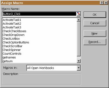
As soon as you release the mouse button a dialog box pops up asking you to choose which macro you wish to associate with this button (illustrated at the top of the next page - Fig 3.2.1). If this is a new worksheet, you won't have any macros waiting to be linked to this button - you have to click CANCEL here. It is easy to associate a macro with this button later.

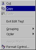
You can customise the appearance of the button (e.g. colour, font, caption) by modifying its properties - try right-clicking the object - a pop-up menu appears (Fig 3.2.2) giving you the choice of a range of common options.

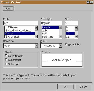
If you select "FORMAT CONTROL" then the standard font dialog appears (Fig 3.2.3) from which you can choose the font face, and other common options.

3.2.2: Check Boxes

Add a group box, label it "CHECK BOXES" and add several check boxes as illustrated below:

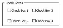
Set the properties of each of the individual check boxes by right-clicking and selecting the FORMAT CONTROL option:

Run through the various tabs on this dialog box, and see what they do. Try a bit of experimentation!

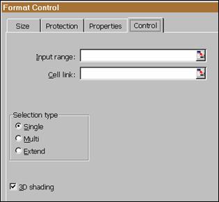
On the "Control" tab (the one illustrated above) check the "3D shading" box, and select a cell on the worksheet as the cell link - this is done by first clicking inside the "Cell link" text area and then selecting the required worksheet cell.

Click OK, and see what happens when you check and un-check the checkbox.

3.2.3 Other Controls

Based upon what we have done above, try adding and using Option Buttons, Scroll bars and Spinners.

3.2.4 List Boxes and Combo Boxes

These controls are used very often, since they provide a convenient method of offering a list of options to the user. First, enter a list of items you want to appear in the list box somewhere in the worksheet - try putting a list of colours in rows 1-5 of column A, for example.

Then draw a list box on a worksheet (it need not be the one containing the list of items):

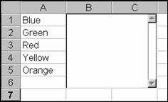
In this example, I have placed the list box next to the list of text items.

If you now right-click the list box, and select FORMAT CONTROL, the dialog box illustrated below will appear. In this dialog box, you need to select the "INPUT RANGE" textbox, and then select cells A1-A5 containing the list items. If you had placed these on a different worksheet, you have to activate that worksheet and again select the relevant cells. Once you have selected these cells the range selected will appear in the open dialog box in the INPUT RANGE textarea.

The next task is to supply a target cell, in the CELL LINK textbox. This is done as before by simply clicking in the target cell.

Try running this example. When you click OK, the dialog box disappears and the text list items appear in the dialog box. You will find that selecting an item in the list causes its list index to appear in the target cell.

The trouble is - it is not the INDEX that we want, it's the text itself! Can you think of a way to do that?

TASK 3.3 - Setting and Retrieving Control Properties and Values using VBA

Draw a group box on your worksheet and fill it with command buttons as shown:

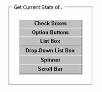
When you draw a command button, a dialog box automatically appears asking you to select a macro to attach to the button. You can't do this until you've written the code, so just click 'Cancel' for now.

We now want to write some code to look at the state of each control - this code will be attached to the buttons shown on the left.

Open the VBA editor, and create a new module to contain the code.

We'll start by adding some code to look at the state of the CheckBoxes:

This code makes use of a number of very useful features of the Excel VBA language. Firstly, you can declare c to be a variable of type 'CheckBox', with a value of 1 meaning 'checked' - look at VBA help under CheckBox. The other useful feature here is the FOR EACH ... NEXT loop, which allows you to look at all objects of a particular type in the context specified - in this case the worksheet named "Task1".

Option Buttons

This is very similar to the above. Have a go a writing a subroutine called CheckOptionButtons and attach it to the second command button in the list on the previous page.

List Boxes and Drop-Down List Boxes

These are slightly different - see the following code:

In this case, we specify the particular listbox we want (we do not want to look at multiple list boxes, if they exist). There is only one listbox on the worksheet, so this is referred to as the first member of the ListBoxes collection. Its Listindex property gives the numerical index (starting at 0) of the item currently selected (-1 if nothing selected) and the List(n) property retrieves the text for the nth item in the list, again starting at 0.

Have a go now at modifying this for the drop-down list box.

Spinners and Scrollbars

After seeing how the values of the other controls have been accessed, these should not prove to be too much of a problem. Here is the code for the spinner:

Sub CheckSpinner()

Dim msg As String

nl = Chr$(10)

With Worksheets("Task1")

n = .Spinners(1).Value

End With

MsgBox "Spinner value is currently: " + Format$(n), 64, "State of Spinner"

End Sub

You can adapt this for the scrollbars. Note that in the example, we have included both horizontal and vertical scrollbars - and that both move together. This is because both have been linked to the same cell.

3.4: Other Tasks

It is rather inconvenient to have to type in the entries for the list box into cells in the worksheet.

3.4.1: Create a text file (using Notepad) containing these entries and save it to disk. Write some code to read in this information and put it in an auto_open macro so that the information is loaded into the list box when the worksheet is opened. (Remember to clear the list first otherwise you will end up with multiple copies of the list items!)

3.4.2: Create a second list (in a second disk file) with some different data. Create an option button group to allow the user to choose which of these two data sets they would like loaded into the list box and write some code to read in data from the appropriate disk file. Attach this macro to the option buttons.

3.4.3: Modify the spinner (or the scroll bar) controls so that they increment the counter by 0.1 instead of 1 each time.

TASK 3.5: Modification of the Example in Task 3.1

Now that we have some experience of using worksheet controls, we can see that we can improve the example presented in Task 3.1 by putting the list of names into a listbox, from which the user can select a name. This is easier to use and less error-prone, so it wins on all counts!

Try writing a VBA program which:

Compiles a list of all the different names in the specified region of the worksheet

Creates a listbox containing these names and places it on the worksheet, in some suitable location (look up the ADD method of the LISTBOXES collection for information on how to do this).

Write a procedure to take a given name and report the total payments to that person, and assign it to the listbox above (look up the ONACTION method).

The macro should be launched using a command button, which should also allow the listbox to be deleted when the user if finished. This can be done by changing the caption of the button. Try giving it an initial caption of GO, which can be changed to STOP (or something similar) while the macro is running. (You can make use of the DELETE method to remove the listbox when finished).

You should try to do this yourself, without reference to the model solution! By all means look at this when you have spent long enough trying to do it yourself, or you need some further help!