PA.1 Sending and Receiving Voltages with the Sending and Receiving VIs
PA.2 Sending and Receiving Voltages from the Front Panel
PA.3 Plotting Measured Samples
PA.4 Using the Autoranging Voltmeter
PA.5 Observing the Oscilloscope Output Graph
PA.6 Discrete Output Voltage from the DAQ
PA.7 Discrete Input Voltage from the Circuit Board
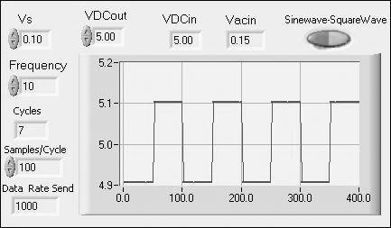
PA.8 Using the Simultaneous Sending/Receiving Function
|
TABLE PA.1 |
||
|
Diagram |
Tools Palette |
Shift/Right Click |
|
Functions Palette |
Right Click-Stickpin to hold |
|
|
Menu Sequence: |
Window>>Show Functions Palette |
|
|
Front Panel |
Tools Palette |
Shift/Right Click |
|
Controls Palette |
Right Click-Stickpin to hold |
|
|
Menu Sequence: |
Windows>>Show Controls Palette |
|
|
Connect Chan0_in directly to Chan0_out o 21321e414v n the circuit board or
connector block. Double Click on both of the
icons in the Diagram of Measure.vi (initial
version) to bring up the VI Front Panels. These are AO Update Channel.vi and AI Acquire Waveform.vi. Set both
In the Front Panel of AO Update Channel.vi, set in a voltage of 1 V or similar (using the Operating Tool). Run the VI, AO Update Channel.vi. To run the VI, use menu sequence Operate>> Run (or, preferred, Ctrl/R). Then run AI Acquire Waveform.vi and note the voltage read (waveform array Digital Indicator). Click on the up and down arrows by the Y to scroll through more data points. Verify that that send and receive are consistent. Try some other voltages. Note the maximum allowed is the highlimit, 10 V. Close the send and receive VIs. Leave Measure.vi open.
|
|
In the Front Panel of Measure.vi (version 2), run the VI (Ctrl/R) with a variety of voltages sent out and verify that the send (output) and read (input) agree. From the Diagram of Measure.vi, Double Click on Mean.vi to open the Front Panel of this VI. Note the X Array Digital Control and the mean Digital Indicator. Now run Measure.vi with Send Volts = 0.1 V. Note that the measurement data appear in the Array Digital Control. These are the data points that are averaged.
Now go to Mean.vi, Right Click on the indicators, select Format and Precision, and type 4 for Digits of Precision. Then scroll through the array data (by clicking on the up and down arrows of the Array Digital Control as shown in the sample) and compare the numbers with the mean. There will probably be some scatter in the least significant digit, due to noise. Note that the number received and averaged is not exactly the same as that requested to be sent out. This is due to the discrete nature of ADC (analog-to-digital conversion) and DAC (digital-to-analog conversion) as discussed and demonstrated in a following section. |
|
Open PlotSamples.vi. Prepare the Diagram for displaying the samples. For high resolution (discussed later), set the high limit and low limit as shown in the example to 1 V and 0 V, respectively. The number of samples can be 10 to 100 and is not critical at this point. We only want to gain some experience with graphs and display the point scatter expected under the conditions set up here. The number of samples is 40 in the example.
Go to the Front Panel to run the VI with the voltage sent out similar to that shown in the example, 0.1 V. This must be lower than the high limit setting for the DAQ input, which is 1 V. At this voltage level, there will certainly be some data scatter. Click on the Y-axis numbers, go to Formatting..., and set the Digits of Precision to 3.
Now run the VI repeatedly. Note that even though there is data scatter, the average value is relatively constant (in the Received Volts Indicator). Note also that the X-axis is in msec. The total time in the graph is 40 times 1 ms (including 0) and AI Acquire Waveform.vi is set for 1000 samples/sec. To set (or verify) the same sample rate as in the example, open the Front Panel of AI Acquire Waveform.vi. Type in the number 1000 for the sample rate and default the value. To default, Right Click on the indicator and go to Data Operations>>Make Current Value Default. Save the VI and close. Re-run the VI with Send Volts = 0.015. Subtract the difference between the measured value of 0.1 V and 0.14 V sent out. Compare the difference with the resolution expected, as obtained from Table PA.2. Note that the high limit is 1V and the mode is Unipolar. |
|
TABLE PA.2 |
||
|
Range |
Resolution |
|
|
Unipolar |
0 to +10V |
2.44 mV |
|
0 to +5V |
1.22 mV |
|
|
0 to +2V |
m V |
|
|
0 to +1V |
m V |
|
|
0 to +500mV |
m V |
|
|
0 to +200mV |
m V |
|
|
0 to +100mV |
m V |
|
|
Bipolar |
-10 to +10V |
4.88mV |
|
-5 to +5V |
2.44mV |
|
|
-2 to +2V |
1.22mV |
|
|
-1 to +1V |
m V |
|
|
-500 to +500mV |
m V |
|
|
-200 to +200mV |
m V |
|
|
-100 to +100mV |
m V |
|
|
-50 to +50mV |
m V |
|
|
Open a new VI in LabVIEW. Then Right Click on the Diagram, and go through Functions>>Select A VI.... and locate ProjectA.llb.
Click on Voltmeter.vi and Click OK. Place the icon on the Diagram. Double Click on the icon to get the Front Panel.
Now place AO Update Channel.vi in the Diagram of your new VI. This is in Functions>>Data Acquisition>>Analog Output.
Double Click on the icon to open the VI. Set the device numbers to match that of your DAQ. Verify that output channel 0 (Chan0_out) is connected directly to input channel 0 (Chan0_in) on the connector block or circuit board. Now run AO Update Channel.vi repeatedly to send out a series of voltages, such as 0.09 V, 0.9 V and 9 V and for each, run Voltmeter.vi. Observe the automatic changing of the limits setting for the various voltages sent out. Note that the voltage is always measured with good precision. Try a negative voltage out. |
|
To run the oscilloscope of Fig. A.14, in the project library, ProjectA.llb, open VI FG_A.vi. (This VI can also conveniently be opened from the Diagram of a new LabVIEW VI.) Then under the Browse menu (from the Front Panel of FG_A.vi) go to Show VI Hierarchy. Locate the icon for OscilloscopeA.vi and Double Click to open the VI.
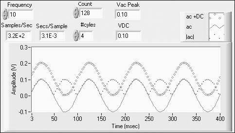
Run FG_A.vi at various values of Vs (Vac peak signal out) and VDCout and observe the combination waveform output in OscilloscopeA.vi. The limit setting is 10 V. The function generator VI, FG_A.vi, is discussed in a following section. |
|
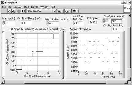
The The VI for assessing the discrete nature of DAQ operation is Discrete.vi. This VI first sweeps the requested voltage to be sent out in a quasi-continuous manner. The programmed sweep increment size is Max Volts/100. For example, for a sweep range of Max Volts = 10 mV, the sweep increments are 100 mV. However, the output voltage has a resolution of 4880 mV (bipolar).
> The receiving function is set with high limit and low limit of magnitude 0.1 V. The resolution for receiving is thus 48.8 mV, that is, much less than the the output voltage steps of magnitude 4880 mV. We will examine, for example, the bipolar mode of the output channels. For this, we need to verify the DAQ configuration for bipolar output. Go to the Start Menu>>Programs>>National Instruments>>Measurements and Automation. (There may be a shortcut for this on the desktop.) Open Devices and Interfaces and then Right Click on the DAQ designator and get Properties.Click on the AO tab and set bipolar. Open Discrete.vi. Verify that Chan0_out is connected directly to Chan0_in on the connector block or circuit board. Verify that in the Front Panel of Discrete.vi, Max Vout is set to 10 mV (for a sweep step size of 100 mV) and that the high limit is set for 0.1 V. Run the VI. The example of this section illustrates what to expect for the case of the DAQ configured for the bipolar mode. Note that the dc offset of the DAQ has been substracted from the plot, such that the measured voltage appears to be zero volts for zero volts sent out. A number for the size of the measured steps is indicated [Vout Step Avg (mV)]. It is obtained by the VI as an average of all the steps. The number shown is expected, as it is twice the DAC reference voltage of Vref = 10V divided by 212 or 2Vref/212 = 4.88mV where the exponent is the number of bits of the DAC. The steps are 2.44 mV for a unipolar output configuration. The graph on the right is a plot of input-channel samples versus sample index. The data illustrate the point scatter due to noise. The noise-free number in the plot at the end of the excution should be 2x4.88 mV = 9.76 mV. Note that the scattered sample points are separated by a discrete value of 48.8 mV. An Array Digital Indicator displays the samples and a Digital Indicator shows the average. Try other full-range sweep values such as Max Out = 20 mV and 5 mV. With Max Out = 10 mV, go to the Diagram and reset the number of samples from 50 to 500. Re-run and note the increased precision, for example, in Chan0_in Array Avg. |
|
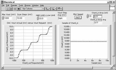
For this measurment, we need a high-resolution output voltage source. If we are willing to give up voltage range, this can be accomplished with a simple resistor voltage divider. In the example here, the circuit forms an apporximate 100:1 divider (270- and 2.7-kW resistors). This provides a source with a resolution of 49 mV (bipolar).
Discrete.vi will be used to investigate the discrete nature of the input channels. Open the VI and set high limit = 0.1 (with low limit = -0.1), for a receiving resolution that is also about 49 mV. Use Max Vout = 1 V (1000 mV). The output voltage sweep range is then Max Vout/100 = 10 mV with the voltage divider. The programmed output voltage step size is Max Vout/100 = 10 mV. Thus, after the voltage divider, this is 100 mV. The resolution of the output and input functions is similar. Run Discrete.vi. The plot is essentially a straight line with similar output and input resolution. Note that the voltage sent out (X-axis) is the actual channel voltage and that the voltage received (Y-axis) is after the voltage divider. Note also that the scatter of the input channel samples (right graph) reflects the discrete nature of the receiving function and the points are separated by about 49 mV. Set high limit = 10 V. Run the VI with the same sweep range (example below). The output voltage (after the voltage divider) has a much higher resolution (better) than the receiving function. The steps in the sweep plot have a magnitude equal to the receiving resolution. Also, the sample points are scattered by the amount of the resolution of about 4.9 mV. An example of this case is shown in Fig. A.18 (Unit A). To check the value of the differences between scattered points, run the VI on SLOW and halt the execution in a transition region. Then step through the Chan0_in Array(mV) Indicator.
The example here illustrates the transition range of voltage between steps; that is, the transition is not abrupt. This is due to noise and the bit uncertainty that exists in the transition regions. Again, the bit-uncertainty effect may be observed during the sweep with Plot Speed set on SLOW. For comparing the two cases with the two limit values and with smoothing of the data with averaging, use AvgDiscrete.vi. This VI runs the subVI Discrete.vi sequentially with the high limit set to 01 and 10 (with the low limit of -0.1 and -10. The two plots appear together in a single graph in the Front Panel of AvgDiscrete.vi. Open AvgDiscrete.vi and Discrete.vi. In AvgDiscrete.vi, verify that Max Out = 1000 mV and that Number Avgs is set at 5 to 10. Run AvgDiscrete.vi to compare the two plots with data smoothing. |
|
With Chan0_out and Chan0_in connected on the circuit board, open FG_A_2.vi. Also open SR_A.vi and OscilloscopeA_2.vi. Open these from Browse>>Show VI Hierarchy. Run the top VI for various Vs and VDCout values. Run the VI at various frequencies and note the change in Cycles and Sample Rate. The number of cycles is increased with frequency automatically to offset delay between sending and receiving. Note the Number of Samples in the array as indicated in the Front Panel of SR_A.vi, for the various changes. Run the VI with SquareWave selected. In the example, VDCout = 5 V and Vs = 0.1 V. There is a slight offset in this example. The oscilloscope's high limit and low limit are set for 10 V and -10 V. Therefore, the resolution is about 5% of the Vs value. There may also be some DAQ offset.
|
|