Introduction to Statistics and SPSS

ISP 121

Activities 6 and 7

Introduction to Statistics and SPSS

Introduction

SPSS (Statistics Package for the Social Sciences) is a software package used for conducting statistical analyses, manipulating data, and generating tables and graphs that summarize data. Statistical analyses include basic descriptive statistics, such as averages and frequencies, to advanced inferential statistics, such as regression, analysis of variance, and facto 141s1817b r analysis.

SPSS for Windows consists of five different windows, each of which is associated with a particular SPSS file type. We will examine two of these windows: the Data Editor and the Output Viewer.

The Data Editor

The Data Editor window displays the contents of the working dataset. It is arranged in a spreadsheet format that contains variables in columns and cases in rows. Notice how there are two tabs at the bottom of the window: Data View, and Variable View.

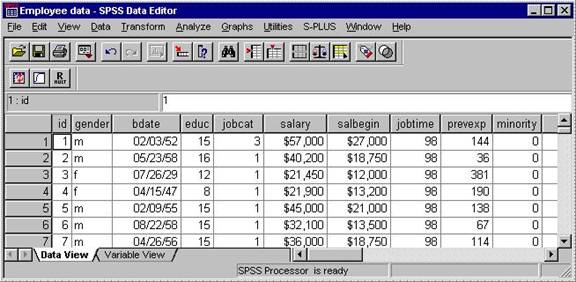
The Data View tab lets you examine the data, much like it appears in an Excel spreadsheet. The Variable View tab allows you to examine information about the dataset that is stored with the dataset.

To import an Excel spreadsheet into SPSS, perform the following:

Copy the file AgeAtInauguration.xls (from the QRC website) to the folder C:\My Documents.

Then, go to Start -> Courseware Applications -> Statistical Applications -> SPSS for Windows -> SPSS 14.0 (or whatever the latest version is) for Windows. (Note: Depending on which lab you are in, SPSS may be in a different location. Check with your instructor.)

Then wait for SPSS to load. This could take several seconds depending upon the lab you are in!

In SPSS, click on File / Open / Data, and select your file C:\My Documents\AgeAtInauguration.xls. Then select Sheet1.

Once the data is loaded, near the bottom of the screen click on the Variable View tab. Do you have a variable named V3? If so, you need to change its type to numeric. You could even rename V3 and the other variables to more useful variable names. Once this is done, click on the Data View tab near the bottom of the screen.

Now at the top of the screen click on Analyze / Descriptive Statistics / Frequencies. You should see the Frequencies window, which looks something like this:

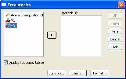
Move the variable V3 to the box on the right side.

Then click on Statistics and make sure the following are selected:

Mean

Median

Standard Deviation

Range

Minimum

Maximum

Click the Continue button to leave this window and then click the OK button in the Frequencies window.

Output Viewer

This should automatically open the Output Viewer with the results you selected and should look something like the following:

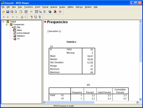
Copy this window into your Word document.

Who was the oldest president at inauguration? Who was the youngest?  (Hey! I always thought John F. Kennedy was the youngest president.  Can you figure out what's going on here?) What does the value Range mean?

How does our current president, George W. Bush, compare to the mean?

How did the previous president, Bill Clinton, compare to the mean?

Can it happen in a dataset that almost every data point is above the average?  Explain why or why not.  If it can, make up an example.

Can it happen in a dataset that almost every data point is above the median?  Explain why or why not.  If it can, make up an example.

Recently we had two of the older presidents (Ronald Reagan, the oldest in history, and George H. W. Bush) but we have also had two of the youngest (John F. Kennedy and Bill Clinton).  Using this data, investigate the question whether presidents inaugurated since 1950 are on average older or younger than the presidents inaugurated before 1950.  Briefly explain your methodology.

Open the file ChicagoBulls1996-97.xls (which contains the salaries of the Chicago Bulls players at the start of the 1996-97 season) in SPSS in the same manner as above. (You'll find it under the "Older data" link at the bottom of the qrc page.) Don't forget to change the salary variable to numeric, as you did above. 

Calculate the mean and median salary and include it in your Word document.

Suppose Michael Jordan had been paid 60 million dollars instead of 30 million.  What would the mean have been in that situation?  What would the median have been in that situation?  (If you used SPSS to do part a, all you have to do is type in 60000000 in place of 30140000 and then run the analysis again.)

Suppose Michael Jordan had been paid 500 million dollars instead of 30 million.  What would the mean have been in that situation?  What would the median have been in that situation?
Because of the property demonstrated in b and c, the median is called a resistant measure because it is not so sensitive to extreme outliers.  Generally, the median is a more realistic measure of the center of a dataset, but it is not always the most useful.  If the distribution of the data is relatively symmetric, then the mean and the median will be close to each other.

Open the file OldFaithful.xls (into SPSS) which contains data on the Old Faithful geyser in Yellowstone National Park.  When this data was collected, the geyser erupted about every hour with some consistency, hence its name.  (It is now erupting about every 1.5 hours.) The file contains data on the length of the eruption and the interval between eruptions. Don't forget to change variable V2 to numeric (and rename it while you are at it).

What is the mean interval between eruptions? (Don't use the duration column, use the interval of eruptions column.)

Make a frequency distribution, or histogram, of the interval data as follows:  When you are in the Frequencies window, click on Charts and then select Histogram. When you examine the output viewer, be sure to paste the histogram (right click on the histogram and copy it) into your Word document.

Part Two

Let's try another example using SPSS. In this example, we will enter our own data and then perform a crosstab, or cross-tabulation. A crosstab allows us to make comparisons of survey data across classifications.  In surveys, the classifications are usually age, race, gender, party affiliation, etc.

For example, let's assume we've asked a number of college students how many drinks it takes before they begin to feel drunk. We also recorded each student's sex and assigned a simple ID. Thus, we might have data that looks like the following:

Gender
ID 1=Female, 2=Male Number of Drinks

11111 1 3

11112 2 4

11113 2 7

11114 1 5

11115 1 2

11116 2 1

11117 2 6

11118 1 4

11119 1 2

We would like to generate for each sex a count of how many said 1 drink made them drunk, 2 drinks, 3 drinks, etc. Thus, we would like to generate something that looks like the following:

Open SPSS and type in the data from the survey. Note: In Data View, you should just enter the data, and not the labels ID, Sex, and Number of Drinks.

Next, go to Variable View. Change the Names of the three variables to something more appropriate, such as ID, Gender, and Drinks. Make sure all variable Types are Numeric. If any of the variables have decimal places, set Decimals to 0.

Then pull down the menu Analyze and click on Descriptive Statistics, then Crosstabs. What variable do you want in the row? The column? When ready, click OK to perform the crosstab. (Hint: ID should not be in either the row or the column. You are not interested in adding up the IDs - you are interested in adding up the number of drinks and the corresponding sex.)

Print or copy the results to your Word document.

Now let's try a little larger example. Let's do a crosstab on the Excel file MCIC-SMOKE.xls.   This file consists of the 1993 and 1997 responses for the question "Do you smoke now?" (SMOKE) along with a set of demographic variables: age (AG), race/ethnicity (RACETH), income level (INC4GP), religious affiliation (REL1), educational level (RESPED), and  gender (SEX01),  Note that the 1993 and 1997 data are on separate pages; there is also a code page that tells you what the codes mean. Familiarize yourself with the codes.

We would like to find out what percentage of men smoked and what percentage of women smoked in the sample in 1997.  The results should produce a diagram that looks something like:

Notice how the numbers add up going down and going across. Using SPSS, create a crosstab and print the results.

Would it be interesting to compare the smoking rate to another variable? For example, which race/ethnicity smokes or does not smoke? Or which income level smokes or does not smoke? Select one of the other variables and produce a crosstab comparing that variable to smoking. Print the results of this crosstab and hand in with above problems.