Rocket Engine Turbopump Flowguide Analysis.

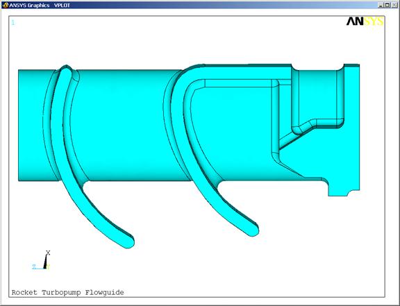
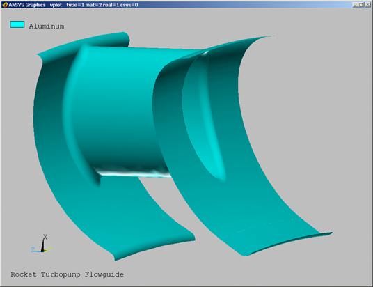
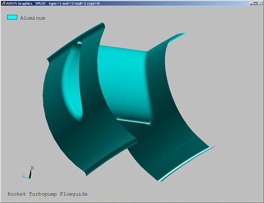
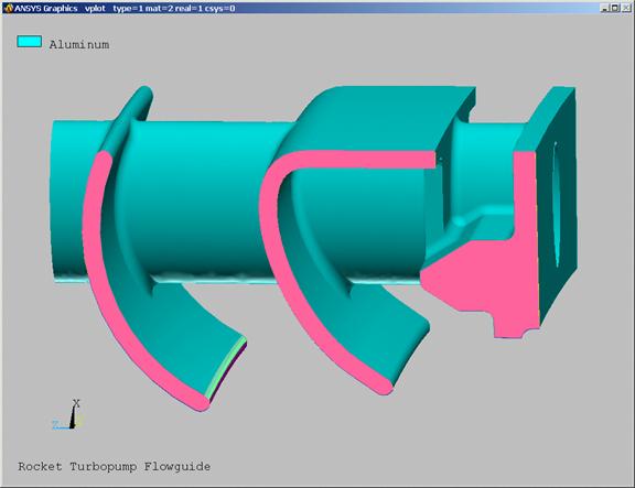
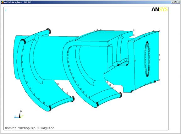
In this exercise, we will perform a thermal transient/static structural analysis of a rocket engine turbo pump flow guide. The flow guide redirects combustion gases through the pump during operation. Before launch, the flow guide is cooled to cryogenic temperatures as liquid oxygen is pumped through it. During launch, the superheated combustion gases heat the flow guide from cryogenic temperatures (-350F) to over 1400F in approximately 10-seconds. Although there are negligible mechanical stresses on the part, thermal gradients are very severe.

The rocket engine is part of a reusable vehicle, which is designed to last for 50 missions. Post flight inspections reveal that the flow guide develops thermo mechanical fatigue (TMF) cracks in the guide vanes after only one flight.

The goal of the analysis is to determine the time point after launch that has the highest thermal gradient through the wall of the flow guide, and perform a stress analysis at this limiting point.

Outline:

Launch ANSYS/Professional with the MTB

Setup Tab:

Model Tab:

Model Import:

Scale Model

Mesh

Mesh Refinement

Thermal B.C.'s

ANSYS/Mechanical Interface

Save model

Launch Classic GUI

Material Properties

Thermal Solution

Solution Options

Initial Conditions

Output Controls

Nonlinear Options

Solve

Thermal Results Post Processing

Plot Model

Define Temp vs. Time variables

Math Operations

Contour Plotting

Structural Modeling

Convert to Structural model

Structural B.C.'s

Temperature Loads

Analysis Options

Structural Solution

Solve

Structural Analysis Post Processing

Stress Plots

Cut Plane Viewing

Animation

Conclusions

Step-by-step Instructions:

Before beginning this problem, create a separate folder on your computer for this job and copy the flowguide Parasolid part file flowguide.x_t to this folder from the InputFiles folder on the CD.

Launch ANSYS/Professional

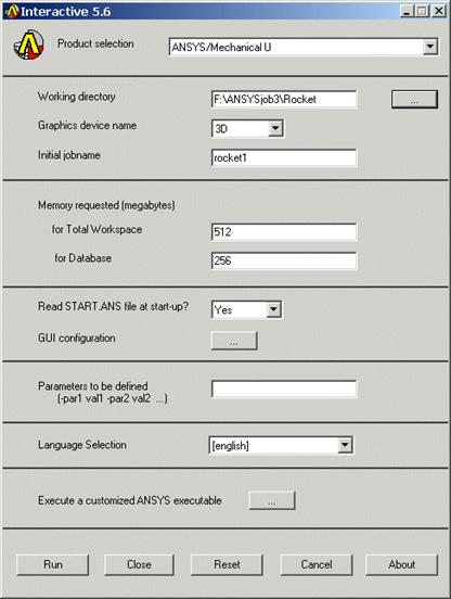
Launch ANSYS using your start menu.

A. Browse to select the working directory you just created for this job.

B. Enter a job name (Rocket1). All ANSYS files created for this problem will have a filename of rocket1 followed by a unique extension.

C. Change the workspace and database sizes for this job to be 512 and 256 respectively.

D. Click RUN to start the ANSYS GUI.

Setup

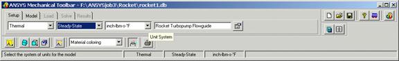
In the Mechanical Toolbar (MTB), we will set the basic analysis type options.

A.

Change Structural to Thermal. Steady-State will be the only available Analysis type.

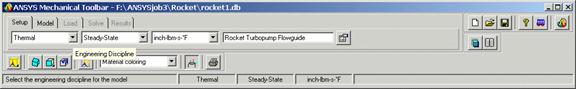
B.

Choose units of Inch-lbm-s-F

C.

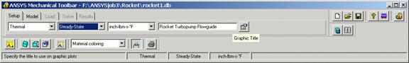
Enter a title for the analysis: Rocket Turbopump Flowguide.

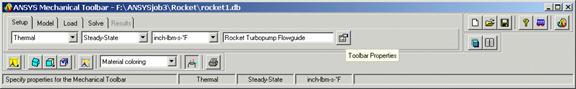
D.

Click on the toolbar properties menu.

E. A menu dialog appears for you to enter menu preferences and other information. Click on the User Info tab.

F. This step is optional. You can enter your name, company name, and address. Click OK when finished.

Model

Under the Model tab, we import the geometry file and mesh the part.

A.

Click on the Model tab in the MTB.

B.

Click on the Import Geometry box to bring up the model import dialog.

C. Change the Files of type: option to Parasolid.

D. In the file list, highlight the file named flowguide.x_t

E.

Click Open.

F. Another dialog box will open asking you to choose import options. Select 3-D Solid.

G. Leave the No model clean-up (faster) option set.

H.

Click OK.

I.

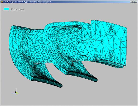
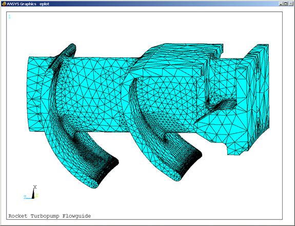
ANSYS will import the Parasolid file and draw the part in the graphics window. Use the dynamic viewing controls to view all portions of the model. This is a 1/22 symmetry segment of the full flow guide.

Scale Model:

Parasolid models like the one we imported usually come from Unigraphics. If a UG model was build in English units (inches), UG converts the file to metric units (meters) when it writes the Parasolid file. When ANSYS imports this file, it has no way of knowing if the originating part was in English or Metric units, so it imports the file as is. In our case, we must convert the file back to English units. This involves scaling it back from meters to inches (multiply by 39.37).

We can perform this scaling by temporarily activating the ANSYS Classic interface.

A. In the ANSYS Utilities Menu, click MenuCtrls:

B. Main Menu:

C. Preprocessor:

D. Operate:

E. Scale:

F. Volumes:

G. Pick All:

H. Enter 39.37 for all three scale factors (RX, RY, RZ).

I. Change the Copied button to Moved. Otherwise you will end up with two brackets, one the original size, and the other the correct scaled size.

J. OK. A warning about ANSYS dialogs: Apply executes the function and leaves the dialog open. OK executes the function and closes the dialog. If you click Apply, it may appear that nothing happened when in fact, your model was scaled. Then, if you click OK, your model will be scaled twice.

K.

The model is now scaled to the correct dimensions. We can turn off the ANSYS input window and return to the MTB. Click MenuCtrls

L. Click on the Main Menu button to turn it off.

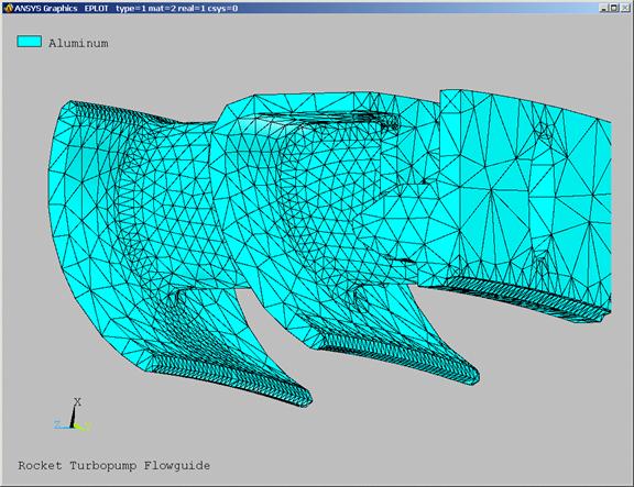
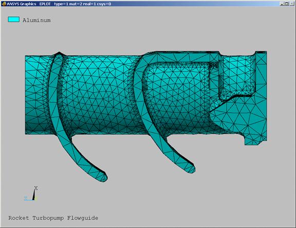
Meshing: We will use the SmartSize meshing to create an initial coarse mesh on the part, then use the MeshTool to illustrate an advanced feature to refine elements at an expected area of interest.

A. The slider bar in the MTB controls the SmartSize mesh density in various levels from very coarse (right most setting) to very fine (left most setting). Drag the slider two notches to the right (coarser setting). This will be the third tick from the right.

B.

Click on the Mesh Model button to create the mesh. This may take a few minutes due to the complexity of the model.

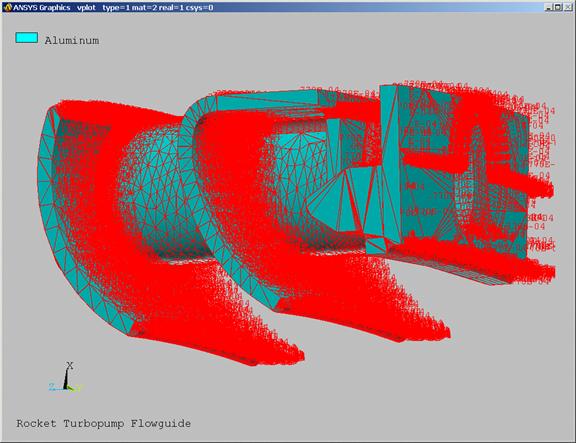
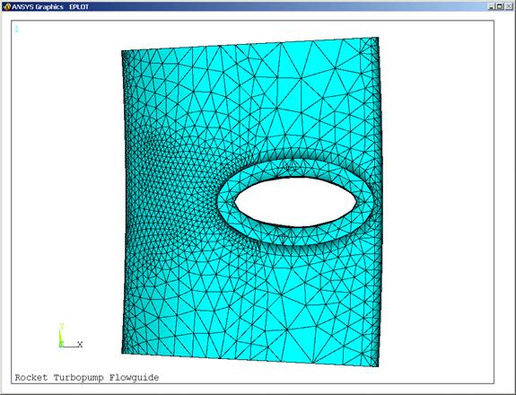
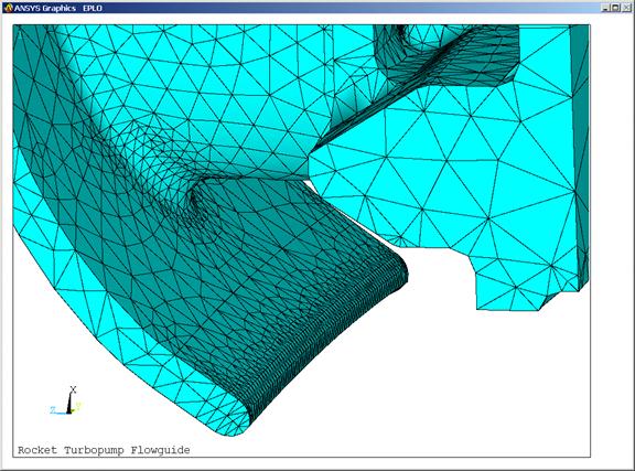
C. A mesh should appear similar to the one shown here. Use the dynamic viewing controls to view all sides of the model. Notice that the SmartSize mesher adjusted the mesh density to be fine in areas of high curvature, or small features.

Mesh Refinement:

Engine test data tells us that the flow guide cracks in the areas shown below. This is caused by the flow guide vanes bending due to the high thermal gradient through them. The mesh in these fillets and the vanes should be refined since they are the areas of interest. We will use some advanced meshing features to refine the mesh in this location.

A.

In the MTB, activate the MeshTool Dialog.

B. A new dialog box will pop up with many advanced features for controlling and refining the mesh. Some of these features are described below:

C. We will use the default feature which is to refine at elements. Other options include refine at volumes, areas, lines, etc.

D. Click the Refine button.

E. A dialog box will appear asking you to select elements for refinement. Click on the Polygon button to activate polygon selection.

F.

Use the Pan/Zoom/Rotate function to orient the model as shown below.

G. Draw polygons shown to select the elements in the lower portion of each vane and the fillet areas between the vanes and main body of the flow guide. Elements are selected when you close each polygon.

H. OK.

I. A dialog box will appear asking you to select the level of refinement. Accept the default (1 minimal) and click OK. ANSYS will refine the mesh. This may take a few minutes.

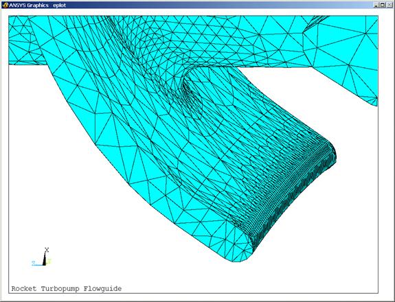
J. Notice how the elements in this region have been refined. Use the Pan/Zoom/Rotate function to see a detailed view of the new mesh.

Thermal Boundary Conditions:

We have completed the model definition phase. The default material assigned by ANSYS is Aluminum and our part is made of a Nickel alloy but we will that alone for now. We will be supplying temperature dependant material properties later on, which must be done in the ANSYS Classic interface.

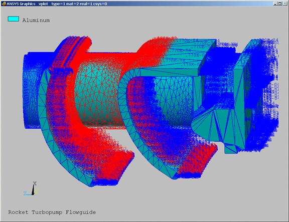
Next we will apply the thermal boundary conditions. There are three unique surface boundary conditions on this model as shown below. The first is a flowpath convection load between the two vanes (purple). All other exposed surfaces (blue) will have a lower convection load. Lastly, the cut boundaries of the flow guide (red) will be adiabatic.

Convection Loads:

A. Click on the Load tab in the MTB. Notice the scrollable box that says Environment 1. As you apply loads and boundary conditions, these will be stored in this load case or "Environment". You can create multiple sets of loads and BC's, each stored in their own Environment.

For thermal analyses, the ANSYS MTB offers four types of boundary conditions that can be applied to the geometry entities (keypoints, lines, or areas). These are enforced temperatures, heat flows, heat flux, or convection loads as shown below. The default is to apply these boundary conditions on areas, but each button has a fly-out menu for you to select other geometric entities for application such as keypoints or lines. The fly-out menus are activated by clicking and holding the mouse over one of the load buttons.

The loads we will apply are shown in the figures below:

Since there are many surfaces on this model and it would be difficult to pick each one, the easiest way to apply the desired loads is by the following procedure:

p     Apply the 77.0e-6 convection load to all surfaces using the pick all button.

p     Apply the 580.0e-6 convection load to the vane flow surfaces. This load will overwrite the previously applied load.

p     The adiabatic surfaces are defined by deleting the convection loads from that surface. Adiabatic is defined as no heat in or out of that surface. This is appropriate for a symmetry surface and is the default for any surface with no boundary conditions applied.

B. Click on the Area Convection button. The default is to apply to areas, so we don't need to activate the fly-out menu.

C. A dialog box will appear asking you to select areas. Click on the pick all button.

D. Enter 77e-6 for the convection load and 1400 for the bulk temperature.

E. OK.

F. ANSYS will draw BC symbols on all surfaces which will make it difficult for you to pick surfaces for the next load condition.

G. We can turn off the symbols by clicking on the Boundary Condition symbol toggle button in the MTB.

We will now apply the convection load to the flow path surfaces. We could pick each area when the convection load application prompts us to, but with this method it is difficult to see all the surfaces to be sure our selection process was correct. Instead, we will use the ANSYS select logic to first isolate all the flow path areas from the rest of the model. This way we can visually see and verify that only the areas we want to apply loads to are selected. The select logic in ANSYS is a very powerful tool that is worth spending some time getting comfortable with.

H. In the ANSYS utilities menu, click the Select button.

I. Click Entities.

J. Change items to select from Nodes to Areas.

K. There are four radio buttons indicating the type of select operation you want to perform. These are described below. We will use the default which is to select From Full.

L. Click the Apply button.

M. A select dialog box will appear for you to select areas. If you click and hold the left mouse button while dragging across the screen, each area to be selected will be highlighted. The area is not actually selected until you release the button. The hot spot for each area is the geometric center, which may not even lie on that area if it is a curved surface like the fillets. You will have to use the dynamic viewing controls to obtain a better orientation for selecting each area. Be sure to pick all areas on both sides of the part. If you accidentally select a wrong area, click the right mouse button. The cursor will change from an upward pointing arrow to a downward pointing arrow indicating that you can now unpick items from the selection with the left mouse button. Click the right button again to toggle back to picking. When you have selected all the areas on the flow path, click OK.

N. Next, click the replot button in the select entities box. Only those entitles which you selected should be displayed. If you did not get all the areas shown in the plot below or have additional areas you don't want, you use the radio buttons to Also Select or Unselect from this set until it is correct. Be sure to replot after selection to verify that the set looks like the one shown below.

After replotting, you should have only the selected areas shown below.

O. Now we can easily apply the convection load to these surfaces. Click the Area Convection button as we did before.

P. Pick All

Q. Enter 580e-6 for the convection coefficient and 1400 for the bulk temperature.

R. OK.

An important point has just been demonstrated here. Every command executed in ANSYS only operates on entities that are selected at the time you issue the command. Even though we said Pick All, the loads were only applied to the selected set of areas. This is a very powerful feature that can be used to simplify modeling, or can lead to error if you are not careful. It is well worth assigning a few brain cells to keeping this thought in active memory.

S. Next, we want to restore all areas to the selected set. In the Utilities menu, pick Select.

T. Everything.

U. Click the Plot Volumes fly-out . The entire model should be restored.

Lastly, the adiabatic or symmetry surfaces must be defined. Adiabatic means no heat in or out of the surface. This is the default condition for any surface that does not have any thermal boundary conditions applied. We will do this by deleting the convection loads from the symmetry surfaces shown in red on the figure at the beginning of section 4.1.

V. Click the Delete BC button in the MTB. This button switches the boundary condition apply functions to delete functions.

W.

Click the Area Convection button.

X.

A new dialog box will appear for you to select areas. Note title at the top of this box that says select areas to delete. convection loads.

Y. Select the three symmetry faces on both sides of the flow guide. These are the red areas in the figure at the top of section 4.1. You will have to use the dynamic viewing controls to select areas on both sides of the part. There should be six areas total. Be sure to get them all.

Z. Click OK.

ANSYS Mechanical:

We have now completed meshing the model and applying the thermal boundary conditions. In order to continue, we will require the functionality of ANSYS/Mechanical to add temperature dependant material properties and to perform the thermal transient solution.

Before proceeding, lets save our work.

A.

Click the save model button in the MTB.

B. Enter a filename of your choice. Rocket1.db will do.

C. Click the Save button.

Enter ANSYS/Mechanical.

A. Click the Fully Functional ANSYS button.

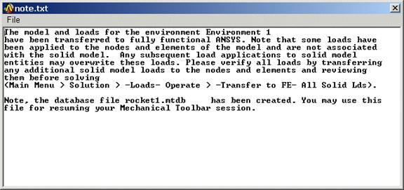
B. A dialog will appear asking you which environment you want to use. This is the set of load conditions we want to preserve. Since we only defined one set of loads or environment, click OK.

C. A warning message will appear indicating that loads have been transferred from the geometry to the nodes and elements and that care must be taken if/when subsequent loads are applied in full ANSYS. Dismiss this warning when you are through reading it.

Material Properties:

Our next step is to define the temperature dependant material properties for the thermal and structural solutions. The properties are listed below:

A. In the ANSYS Main Menu, click Preprocessor

B. Material Props

C. Material Models.

D. A material property dialog will appear for you to select the type of properties you want to define. Under Material Models Defined, there are four models predefined for you by the ANSYS Mechanical Toolbar. Our flowguide model references the lowest property ID of 1. We will redefine the properties for this model.

E. Pick Structural

F. Linear

G. Elastic

H. Isotropic

I.

A dialog box will appear for you to enter the linear elastic structural properties of modulus and poison's ratio. The temperature field is grayed out by default, which assumes that your properties are not temperature dependant. Click the Add Temperature button and another column will appear with the temperature fields now active.

J. Enter the modulus and poisson's ratio data for the first two temperatures as shown below. You will overwrite the existing data.

K. With the cursor still positioned in one of the cells of column T2, click the Add Temperature button.

L. A new temperature column will be added after column T2. Had the cursor been positioned in column T1 when you clicked the Add Temperature button, the new column would have been positioned between the two columns you just filled with data. Continue adding data for the next temperature (70 degrees).

M.

Click the Add Temperature button again and repeat the procedure until you have entered all the modulus and poisson's ratio data in the table at the beginning of this section.

N. After the data has been entered for all 8 temperatures, pick the Graph button click over the Ex field.

O.

A plot of the modulus data will appear.

P. Pick OK in the material input dialog.

OK, I know what you're thinking. Remain Calm! We're not going to make you do this again four more times for the other property tables. ANSYS has the ability for you to create your own materials database. We created one for the stainless steel you are using in this problem. All you have to do is import it.

Q. In the Materials Property Dialog, Click Material Library

R. Import Library

S. Select BIN for the units.

T.

OK

U. Change the material ID number to 1

V. Depending on your system, you may have to select the drive and location to your working directory where this file is stored.

W. Highlight the stainless.bin_mpl file.

X. OK

You can create material data files yourself using a text editor, or by inputing properties through the menu like we just did, and exporting them to a database file.

Y. The properties will be listed for you in a list window. Close this window when you are through reviewing the properties.

Thermal Solution:

Thermal Solution Options:

We have completed the model definition, boundary conditions, and material property definition for the thermal solution. Now we must set some of the nonlinear solution options before solving the thermal transient solution.

A. Enter the Solution module by clicking on Solution in the ANSYS Main Menu.

B. Click the New Analysis button.

C. In the dialog that appears, select Transient Analysis.

D. OK

E. Another dialog will appear for you to choose solution method. The default is Full Newton Raphson method which we will accept.

F. OK

G. In the Solution menu, click Fast Sol'n Optn.

H.

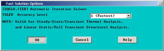
Accept the default which is Fastest. OK.

Initial Conditions:

A. Next, we will assign initial conditions for the thermal analysis. This is simply the starting temperature for the analysis. The flow guide is initially at -350 degrees which is the initial condition. In the Solution menu under -Loads- pick Apply.

B. Initial Condit'n

C. Define

D. Pick All

E. Select TEMP

F. Enter -350

G. OK.

Output Controls:

A. Next we want to select results file output controls for the solution. By default, ANSYS stores output temperature, heat flux, and nodal gradient results for the last step in a solution. For our analysis, we only require nodal temperatures, and we want them for every substep in the transient. In the Solution menu under -Load Step Opts- pick Output Ctrls

B. DB/Results File

C. The settings you apply in this dialog box are cumulative, meaning that anything you select is added to the current setting. In order to write nodal temperatures ONLY, we must first turn off all existing settings and then add what we want. Select the None button. This will suppress all items.

D. Apply

E. Next, select Nodal DOF Solu from the items to be controlled list.

F. Select Every substep

G. OK.

Time Step Options.

Lastly we need to set the time step options. The ANSYS automatic solution control could be used as is to set the initial, minimum and maximum time steps sizes to obtain the solution. However, the program would perform several restarts until it determines the appropriate time step sizes for this problem, and thus waste a lot of CPU time. This feature is valuable when you solve a new class of problems and don't know what settings are appropriate. As you gain an understanding of your typical problems, you will find that you can speed solution by wisely choosing the initial settings. To speed solution, we will provide you with the best settings.

Again, these settings are dependant on the class of problem and are usually obtained through trial and error.

A. Select Time/Frequency in the Solution menu.

B. Time - Time Step.

C. Enter 10 as the ending time in the analysis.

D.

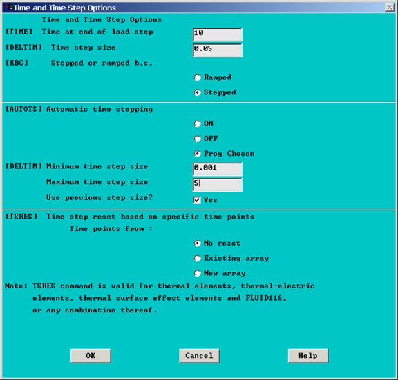
Set the initial time step size to 0.05

E. Choose Stepped loading. This means that the boundary conditions are applied at their full value throughout the entire loadstep. The default (ramped) loading condition means that the loads are ramped up to their full value starting from zero.

F. Enter the minimum time step value as 0.001.

G. Enter the maximum time step value as 5.

H. OK

Solve thermal transient.

A. We are now ready to perform the thermal transient solution. Before continuing, lets save our work. In the ANSYS Utility menu, pick File

B. Save as jobname.db

C. In the Solution menu under -Solve- pick Current LS.

D. A dialog box will appear showing the current solution options you selected. Take a moment to verify that your settings match what is shown below. Dismiss this window when you are finished reviewing it.

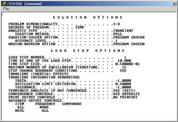
E. Click OK to begin the solution.

F. A dialog box will appear notifying you of any warning messages and asking if you want to proceed. Click OK. The nonlinear solution may take several minutes. During solution, the graphics window will track time stepping and convergence norm so you can monitor the progress.

G. A window will appear notifying you that the solution is done. Click Close.

Thermal Solution Post Processing

Plot Model.

A. Before we begin post processing, lets replot our model. The plotting controls in the Classic menu are in the Utility menu. Click Plot.

B. Elements

C. The model should appear in the default front view.

D. The Pan/Zoom/Rotate function is also located in the Utilities menu. Pick PlotCtrls

E. Pan/Zoom/Rotate

F.

The pan/zoom/rotate dialog will appear.

G. Use the Pan/Zoom/Rotate to orient the model as shown below.

H.

Zoom in on the forward vane section as shown below:

We are now ready to post process the thermal solution. The maximum stresses in the flow guide occur when the thermal gradient is the highest through the wall of the forward vane. We want to calculate this thermal gradient and plot it as a function of time throughout the 10 second start transient. We can do this in the Time History Post Processor.

Define Nodal Variables

The Time History Post Processor is used for tracking variables across time. It is used to evaluate nonlinear solution results throughout the time domain. This differs from the General Post processor which is used to evaluate results at a descrete point in time.

We will define three variables in the Time History Postprocessor: The temperature on the vane flowpath surface, the temperature on the vane inside surface, and the Delta between them.

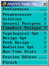
A. In the ANSYS main menu, select TimeHist Postpro

B. Define Variables

C. Add Note that in this dialog, variable 1 for Time has already been predefined for you. This is a vector containing all the time values from your solution.

D. Nodal DOF Result

E. OK

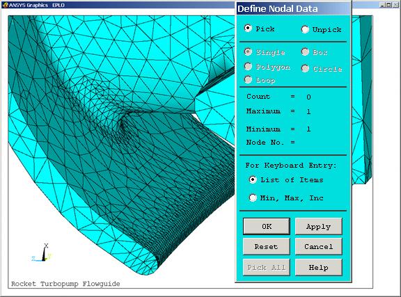
F. A dialog box will appear for you to select a node for the first variable.

G. Pick a node on the vane flow path surface.

H.

OK.

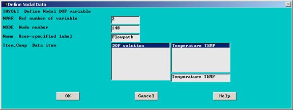
I. A dialog box appears for you to define a label for this variable, and what data to associate with it. Enter Flowpath for the label.

J. Temperature is your only option for data.

K. OK. ANSYS just defined variable 2 for you, which is the temperature at the node on the flowpath surface.

L. Pick Add again to add the second variable.

M. Nodal DOF is highlighted again. Pick OK

N. Pick the node on the inside vane surface opposite the flowpath node we previously selected.

O. OK

P. Enter a descriptive label for this variable: Inside

Q. OK

R. We now have three variables defined as shown below. The predefined variable number 1 is time, 2 is the Flowpath surface temperature, and 3 is the inside surface temperature.

S. Close this dialog.

Math Operations:

Next, we will define the most important variable, which is the difference between the flowpath temperature (variable 2) and the inside surface temperature (variable 3).

A. In the TimeHist PostPro menu, Pick Math Operations

B. ADD

C. A rather intimidating dialog box will appear for you to define a new variable. You will be defining terms of the equation listed at the top of this dialog box. Note that ANSYS is using the variable numbers. for this equation. You just defined two of them where 2 is the flowpath temperature, and 3 is the inside surface temperature. We will define a new variable 4 (next available), which will be the difference between variables 2 and 3. For Reference number for result, enter 4.

D. For 1^st variable, enter variable number 2 (flowpath temperature).

E. For FACTB, enter -1. This will subtract the second variable.

F. For 2^nd variable, enter variable number 3 (inside surface temperature).

G. For the user specified label, enter Delta-T

H. OK

I. We can now list and graph these variables as a function of time. Select Graph Variables from the TimeHist PostProc menu.

J. In the dialog that appears, enter 2, 3, and 4 as variables to graph. These will be plotted against variable 1 which is the predefined time variable.

K. OK

L.

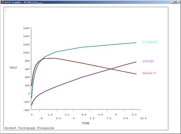
The three variables will be plotted as a function of time. Note that the maximum Delta-T occurs somewhere between 2-3 seconds.

M. We can list these values to more accurately identify the worst time. In the TimeHist Postproc menu, click List Variables.

N. Enter variables 2, 3, and 4.

O. OK.

P. In the list window, make a note of the time at which the maximum Delta-T occurs. In the example below, it is Time 2.31. (Your time may be slightly different).

Q. Close the List window when you are through studying it.

Temperature Contour plot and Animation over time.

Now that we have determined the worst time point, lets plot the temperatures at this time and also animate the temperatures over the entire mission.

A. In the Main menu, Select General PostProc.

B. Results Summary

C. Note that you have results from approximately 11 time points. Make a note of the set number in this list. In the example below, this is 8. (Yours may be different).

D. Close.

E. Under -Read Results- pick By Set Number

F. For Data set number, enter 8

G.

OK

H. Temperature results have now been loaded into memory. Select Plot Results

I.

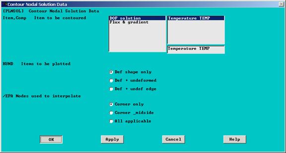
Nodal Solu.

J. Temperatures are already highlighted since that is the only result quantity we saved. Pick OK

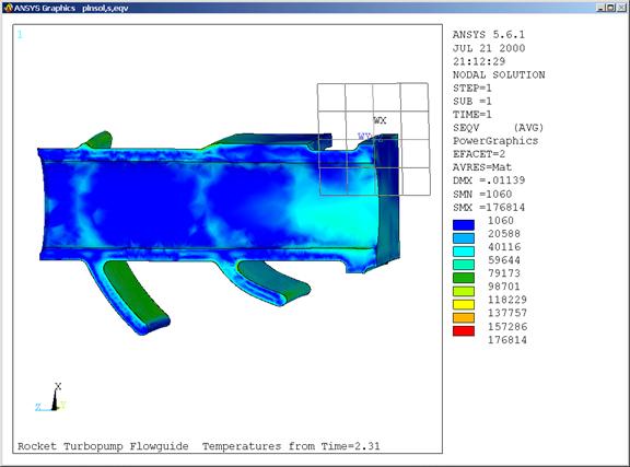
K.

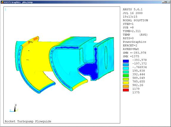
Use the Pan/Zoom/Rotate function to view all portions of the model. Note that some portions of model do not show smooth contours. This is due to the coarse mesh density, and the ANSYS default setting which is to plot results only at the corner nodes. The latter setting can be changed, but we won't bother here.

L. Lastly, lets animate the temperatures throughout the 10 second mission. In the utility menu, pick PlotCtrls

M. Animate

N. Over Time

O. You can choose the number of animation frames and load step or time step range for animation, and the results quantity. In our case, just accept the defaults by picking OK.

P. The animation will be generated and displayed by your systems video player. Click the image below for an example.

Stress Solution:

We are ready to perform the Mechanical stress solution. The procedure is to convert our finite elements from thermal to structural elements, load in the temperatures as thermal loads, apply the mechanical boundary conditions, and solve the stress solution.

Switch Element Types

A.

In the ANSYS Main Menu, Pick PreProcessor

B. Element Type

C. Switch Elem Type

D. Select Thermal to Struc

E. OK

F.

A warning will appear for you to check element settings and other model info. Close the box when you are through reading it.

Structural Boundary Conditions:

We will now apply the symmetry boundary conditions to restrain the model. The front face of the flow guide is bolted to mating turbine hardware. The bolt holes are not modeled since they are not relevant to this analysis. We will restrain the entire front face for simplicity, along with the symmetry cut faces.

A.

In the ANSYS Main Menu, Pick Solution:

B. Under -Loads- pick Apply

C. Displacement

D. Under -Symmetry B.C.- pick On Areas

E. Select the areas shown in purple in the figure below. Be sure to select the cut faces on both sides of the model. There will be 7 areas total. For symmetry boundary conditions, ANSYS will restrain the degrees of freedom normal to the surface of model.

F. OK

G. In the Utilities Menu, Pick Plot

H. Areas

I. You should see symmetry symbols on the areas you selected.

Apply thermal loads.

We will apply the thermal boundary conditions from our previous thermal transient solution.

A. In the solution menu under -Loads- Pick Apply

B. Temperature

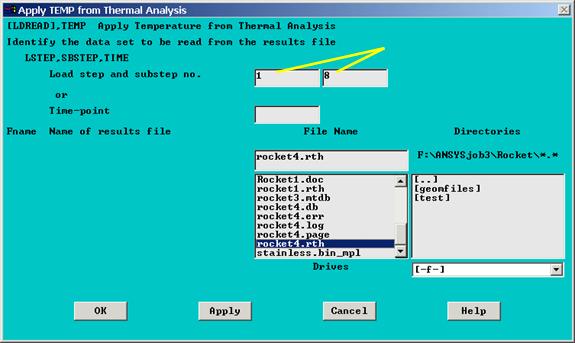
C. From Thermal Analy

D. In the dialog box that appears, you can identify the time point from the thermal solution either by load step and substep number or by the actual time value. In the example shown below, we enter Load step 1, and substep 8.

E. Choose the result file, which will be your jobname with a .rth extension. In our case, this should be rocket1.rth

F. OK

Analysis Options.

We will need to set some analysis options before performing the solution.

A. We will now be performing a linear static stress solution, which is the default type of analysis in ANSYS. In the solution menu, pick New Analysis

B. Change Transient to Static

C. OK

D. Close the warning dialog.

E. All the other settings (time step options, results file output controls, etc.) need to be reset to their default options which is appropriate for a linear static analysis. We can do this with one reset command. In the Solution menu under -Load Step Opts- pick Reset Options...

F.

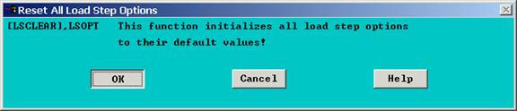
OK

G. Lets change the title for the analysis to identify the condition we are analyzing. In the Utility menu, pick File.

H. Change Title

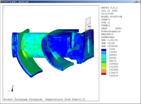
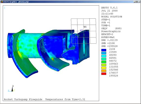
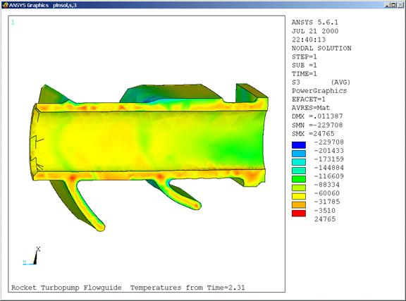
I. Enter a descriptive title: Rocket Turbopump Flowguide. Temperatures from Time=2.31

J. OK

Structural Solution.

Solve

A. We are ready to perform the structural solution. Before doing so, lets save our work. In the Utilities menu, pick File

B. Save as Jobname.db

C. In the solution menu under -Solve- pick Current LS

D. A status window will appear. Note that all the load step options and output controls have been reset for a linear static solution as shown below. Dismiss this window when you are finished reading it.

E. OK. The solution may take several minutes.

F. A dialog box will appear indicating that the solution is complete. Pick Close to dismiss this box.

Structural Analysis Post Processing:

In the post processor, we will review the von mises stress and the principal stresses. We will also use some advanced graphics features to view a section plot of the internal hole through the flow guide.

Enter the General Post Procesor

A. In the Main menu, pick General Postproc.

B. Plot Results

C. Nodal Solu.

D. Choose Stress and von Mises SEQV from the menu.

E. Apply Use Pan/Zoom/Rotate function to view all portions of the model.

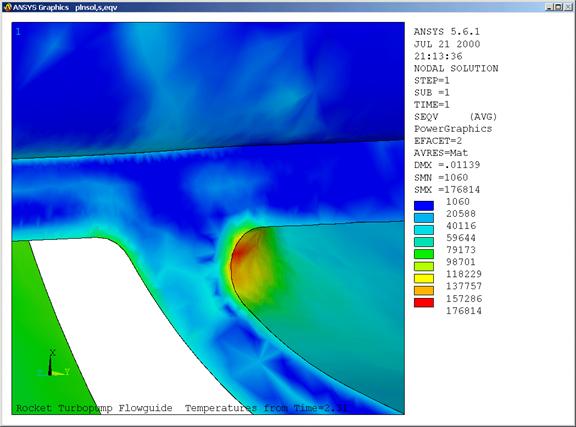
F. Notice the high stress areas in the lower fillet between the forward vane and the body of the flow guide. What is causing this stress to be so high?

Since the flow path surface of the vane heats up faster than the inner surface, it tends to expand more than the inner surface, which creates a bending condition that is reacted out at this fillet location.

G. Notice the high stress in the top fillet between the vane and main body. What is causing this stress concentration?

You should have noticed by now the spotty nature of the stress contours. We would expect the stress distribution to be smooth. What does this tell us about our model? Stress gradients are very high due to the extreme temperature gradients in the part. Remember from the thermal analysis that the gradient through the vane wall was well over 800 degrees. Our vane wall has at most two elements through the thickness. Is this adequate to capture the stress field accurately? Probably not, but it is good enough to capture the general response of the part under these conditions. You will notice in the plots to come that many regions need mesh refinement.

If we were calculating the LCF life or strength margins on this part, we should probably repeat the analysis with a much finer mesh. That, of coarse, would require much longer run times and greater computer resources.

Cut Plane Viewing

Much of the surface area of the flow guide is hidden from view due to its hollow nature. We can use some advanced graphics plotting to create a cut plane view to reveal the inner surfaces of the part. Next we will orient the ANSYS Working Plane to graphically split the flow guide in half for better viewing.

A. Reorient the viewing area as shown in the plot below. In the ANSYS utility menu, pick WorkPlane

B. Display Working Plane.

C. The Work Plane will be drawn as a small grid. Notice that it is currently oriented on the plane of the front face of the flow guide.

D. We want to orient this work plane so that it cuts the flow guide in half long ways. Note that the triad on the workplane grid indicates that the X-axis is pointing up. If we can rotate the working plane 90-degrees about it's X-axis, it will be positioned correctly. In the Utility menu, pick WorkPlane again.

E. Offset WP by Increments.

F. A dialog will appear that looks very similar to the Pan/Zoom/Rotate dialog. The functions are the same, except that these options operate on the work plane instead of the view.

G. In order to rotate the work plane 90 degrees about the X-axis, you can either drag the degree slider bar over to 90-degrees, then click the +X button, or leave the slider set at 30-degrees and click the +X button 3 times.

H. Do so now and orient the work plane as shown in the plot below.

I. Now we are ready to do a capped plot, which graphically removes the portion of the model on the +Z side of the cutting plane. In the Utilities menu, pick PlotCtrls

J. Style

K. Hidden Line options.

L.

Select Capped Z-buffer for type of plot.

M. For the cutting plane, select Working Plane.

N. OK.

Use the Pan/Zoom/Rotate function to view all sides of the model. What does the capped view tell us about the stress field in the model?

O.

The plot should look like the one below.

P. In the Utilities menu, pick WorkPlane and Display Working Plane again to toggle the work plane grid display off.

Q. Note the high stress location in the lower vane fillet. From the capped view plot, we can see that this stress is very local in nature and dies out very quickly through the thickness of the part. What does that tell us? The stress is dominated by bending.

R. Lets view the principal stresses in order to see which locations are in tension and compression. In the Postprocessing menu, pick Plot Results.

S. Nodal Solu.

T. Pick Stress and 1^st Principal S1

U. OK. Notice the high tensile principal stress on the forward inside wall of the flow guide body. We would not be able to see this stress without using the capped view plot.

V. Next, plot the min principal stress which is the 3^rd Principal Stress S3. Note that the high Von Mises stress in the lower vane fillet is actually a compressive stress. What does that tell us? The vane must be bending inward.

Animation:

A.

Lastly, let's animate the stress results to better visualize how the bracket deforms during loading. Before doing so, use the Pan/Zoom/Rotate function to obtain a view suitable to see the entire part. Your current view settings will be used to generate the animation movie.

B. In the ANSYS Utliities Menu, click on PlotCtrls

C. Animate

D. Deformed Results.

E. Stress

F. VonMises SEQV

G. OK

H.

This may take a few minutes while ANSYS generates animation segments and launches the animation in your media player. Click the image below to view an animated von Mises plot.

Conclusions:

What have we learned about the design? The thermal loads on the part induce a high compressive stress in the vane fillets. How could we reduce this stress? What would be the effect of thickening the vane or increasing the fillet radius?

Since the stresses are primarily driven by thermal gradients, increasing wall the wall thickness would actually aggravate the problem by increasing the thermal gradient. We could probably reduce the stresses by decreasing the wall thickness. What other measures could be taken? What about changing materials to a lower alpha alloy? What other shape changes would help?

Are there other analyses might be necessary to verify this design? Could other time points in the mission produce higher stresses in other areas?

Congratulations! You are now a Rocket Scientist.