Suppose you want to develop an Excel application that allows a user to enter details of a loan and to explore various repayment options (i.e. prices, interest rates, repayment periods etc) but to prevent the opportunity for mistakes in data entry. Excel has some powerful tools to help you do this.
When you interact with Excel you are using its graphical user interface (GUI) , which consists of menus, dialog boxes, list boxes and other controls. The idea is to make the application easy to use, and to reduce errors by restricting choices to valid options.
In Excel, you can create your own GUI by utilising the ActiveX controls 10210i81k in the control toolbox. In many cases, you can create an application without any programming at all.
Open a new workbook in Excel, and enter the following labels into the cells shown. This will indicate the data required by the loan payment model.
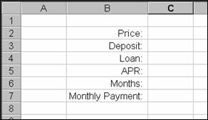
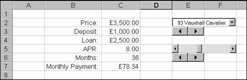
Cells B2-B7 contain labels for the required items: the user should enter the price, the deposit, the APR and the length of the loan in months, and the program should determine the amount of the loan and the resulting monthly payment.
Go through the following steps to create a fully functional loan payment calculator.
Format cells C2, C3, C4 and C7 as Currency. (Right-click the cell and select Format from the menu)
Type 5,000 into cell C2 and 1,000 into cell C3. Type 8 into cell C5 and 36 into cell C6.
In Cell C4 type =C2-C3
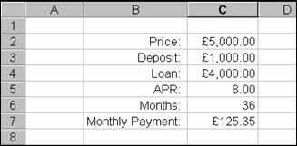
In Cell C7 type: = -PMT(C5/100/12,C6,C4) If you want to see how to use this function, check the help file. Briefly, the first argument is the monthly
interest rate, the second is the number of payments, and the third is the total
loan amount). This example makes an
incorrect assumption - that the monthly interest rate is one twelfth of the
yearly interest rate. We'll deal with
that later - remember for now that what we have done is an approximation.
You can try changing the details of the loan to see how the monthly payment responds.
One of the problems of this model is that it allows too much flexibility - you can enter nonsensical values such as interest rates of 500% or "balloon". This is where worksheet controls come in!
Creating a Error-Free Loan Calculator
The idea here is to restrict the user's choice in what they enter for the various items. Display the Control Toolbox - this has the tools we need.
Restrict the number of months to a valid range
Suppose we feel that a suitable range is 12-60 months (1-5 years). We can use a spin button to control this. Having activated the control toolbox (click the control toolbox button on the Visual Basic toolbar):
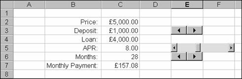
Click the Spin button control. Hold down the ALT key and click close to the top-left corner of cell E6 (the ALT key snaps the control to the grid cells). While holding down the ALT key, drag the mouse to the bottom-right of cell E6 and the release the mouse and the key.

You should find that a spinner control has replaced cell E6:
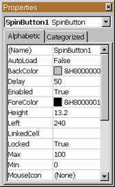
Right-click the spinner and select Properties to display the Properties window
(or use the 2nd button on the control toolbox). Change the Max and Min properties to 60 and
12, respectively. For the LinkedCell,
type C6, and press Enter.
Click the Exit design mode button and test the spin button out.
Repeat this for the Deposit entry field. You will need to also set the SmallChange property of the spinner control - otherwise it would take a long time to spin from 1,000 to 2,000 for example!
Restrict the interest rate to valid values.
This is expressed as a percentage, and will be restricted to lie between 0 and 20%. We will aim to allow the value to be changed in steps of 0.25%. For variety, let's use a scroll bar here.
Add a scroll bar from the toolbox to cell E5. You will find that you can only set the value of this control (like the spinner) in integers, so to arrange for the value that appears in cell C5 to vary in steps of 0.25 we need to use an intermediate value.
In the Properties window for this control, set the Max property to 80 and set the SmallChange and LargeChange properties to 1 and 8 respectively. Set H5 to be the value of the LinkedCell property. Press ENTER.
Exit design mode and test the control. You will find that clicking on one of the arrows at the end of the scrollbar changes the contents of cell H5 by 1, while clicking inside the bar changes the value by 8.
Enter the formula =H5/4 into cell C5. You should now find that the scroll bar does the correct thing.
Retrieving a Value from a List
You could specify the price of the item being purchased using another scroll bar, but let us suppose we are buying a car. The price is determined by the exact car you want to buy, and you may have a list of available cars along with their prices. You can make the loan model user-friendly by providing a pick-list of cars to choose from.
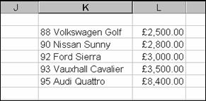
Suppose the relevant information is stored in a list starting in cell
We now want to add this information to a drop-down list box. From the control toolbox, select the combobox button and draw a box over cells E2 & F2.
Set the Style property to 2 - frmStyleDropDownList. Enter C2 as the LinkedCell, and K2-L6 as the ListFillRange. Click Exit Design Mode and check the operation of the list control.
You will notice that the list box puts the entire contents of the selected listbox row into cell C2, not just the price. To do this, go back to the listbox properties, and enter 2 for the ColumnCount property, and 2 for the BoundColumn property.
Exit Design Mode again, and re-check the operation of the listbox. You should find it now works OK.
The drop-down list box now works fine, however while the list was dropped down there was a horizontal scroll bar across the bottom. Even though there is plenty of room for the price, the combo box makes the price column just as wide as the car name column. To correct this you need to experiment both with the overall width of the combobox, and with the ColumnWidths property of the listbox.
To set the latter, try typing 100;36 for the widths of column 1 and 2 (in points, 72=1"). Try also making the listbox span 3 cells. You should find that works OK.
Protecting the Worksheet
This application now works find, and does not require any typing into cells (and you did it with no macros!). However, there is nothing to stop a user typing something into the cells.
You can protect the worksheet, but doing this in the usual way would prevent your worksheet controls from functioning also. You can, however, set the worksheet protection in such a way that Visual Basic procedures can still change the contents of the cells. You need to create a simple event handler for each of the controls. In essence, protecting the worksheet stops the "LinkedCell" property from functioning - you need to reproduce this effect with a VBA line of code.
Create an event handler for the combo box.
Here we convert the ActiveX controls from linking to the cells, to using an event handler to put the new value into the cell.
Turn on design mode and select the combo box.
Rename the control cboPrice. (the prefix is just to denote the type of control - it's not essential).
Clear the LinkedCell property box and click the View Code button on the control toolbox (or double-click it). A new event handler procedure called cboPrice_Change appears. Change is the default event for a combo box.
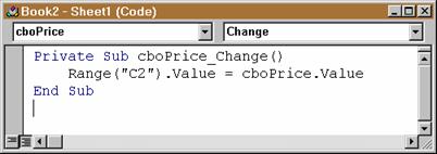
Type into it the line: Range("C2").Value = cboPrice.Value
This will change the contents of C2 to the new value in the combo box whenever tat value changes.
Repeat steps 1-4 above for the spin button and scrollbar controls. Name the controls spnDeposit, spnMonths and scrRate, and use these lines of code where appropriate:
Private Sub spndeposit_Change()
Range("C3").Value=spnDeposit.Value
End Sub
Private Sub spnMonths_Change()
Range("C6").Value=spnMonths.Value
End Sub
Private Sub scrRate_Change()
Range("C5").Value=scrRate.Value/4
End Sub
Clear cells H5 and H3 - you don't need them any more.
You now have an event handler procedure for each control and none are linked to worksheet cells. You are ready to protect the worksheet!
Protect the Worksheet
You typically protect the worksheet by clicking the protection command from the Tools menu and then clicking the Protect Sheet command. Doing this means you can't subsequently modify the sheet in any way (not even with a macro!).
A macro can, however, protect a sheet in such a way that a macro can still change locked cells. This special kind of protection does not last when you close and re-open a workbook, so you must protect the worksheet each time the workbook is opened. As seen in the last tutorial sheet, we can use the Workbook_Open event to do this.
Activate the VBA editor, click the Project Explorer button and double-click the ThisWorkbook object.
Select Workbook from the object list.
Place this code in the Workbook_Open procedure:
Sheets("xxx").Protect UserInterfaceOnly:=True
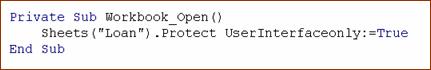
The UserInterfaceOnly argument to the Protect method is what allows a macro to make changes even when a user or a control cannot.
Save and close the workbook, then re-open it.
Test it out!
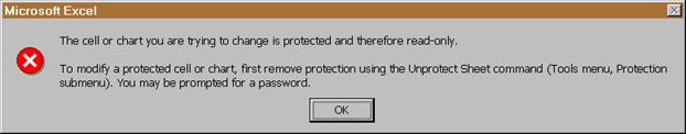
Try typing numbers into the worksheet. This is what happens.
|