A CFD Analysis - Step By Step
Use the information in the problem description and the steps below as a guideline in solving the problem on your own. Or, you can use the detailed interactive step-by-step solution that follows.
Preprocessing (Laminar Analysis)
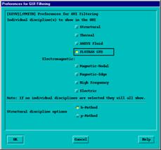
Set preferences.
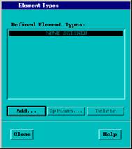
Define element type.
Create rectangle for the inlet region.
Create the outlet rectangle.
Create the transition region between the rectangles.
Establish mesh patterns.
Create the finite element mesh.
Create command on the Toolbar.
Apply boundary conditions.
Solution (Laminar Analysis)
Establish fluid properties.
Set execution controls.
Change reference conditions.
Execute FLOTRAN solution.
Postprocessing (Laminar Analysis)
Read in the results for postprocessing.
Plot velocity vectors.
Plot total pressure contours.
Animate velocity of t 333i81d race particles.
Make a path plot of the velocity through the outlet.
Solution (Laminar Analysis with Change in Inlet Velocity)
Increase the inlet velocity.
Run the analysis.
Postprocessing (Laminar Analysis Using New Inlet Velocity)
Plot total pressure contours.
Animate velocity of t 333i81d race particles.
Make a path plot of the velocity through the outlet.
Preprocessing (Laminar Analysis with Increase in Duct Length)
Delete pressure boundary condition.
Construct additional outlet region.
Establish mesh divisions for the new rectangle and mesh.
Apply boundary conditions on new region.
Solution (Laminar Analysis Using New Duct Length)
Change the jobname and execute solution.
Postprocessing (Laminar Analysis Using New Duct Length)
Read in the new results and plot velocity vectors.
Plot total pressure contours.
Animate velocity of t 333i81d race particles.
Make a path plot of the velocity through the outlet.
Calculate Reynolds number.
Solution (Turbulent Analysis)
Specify FLOTRAN solution options and execution controls.
Rerun the analysis.
Postprocessing (Turbulent Analysis)
Plot total pressure contours.
Animate velocity of t 333i81d race particles.
Make a path plot of the velocity through the outlet.
Exit the ANSYS program.
Detailed descriptions of all of these steps follow the problem specification and description below.
This problem models air flow in a two-dimensional duct. First,
an arbitrary inlet velocity is defined initially to simulate laminar flow with
a Reynolds number of 90. After the solution is obtained and examined, the inlet
velocity is increased to investigate its effects on the flow profile and a new
solution is obtained. Then, in the third part, the duct length is increased to
allow the flow to achieve a fully developed profile in the solution. Finally,
after calculating that the Reynold's number is greater than 4000, a new
solution is restarted using the turbulent model.
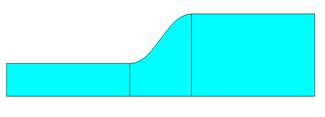
|
Dimensions & Properties |
|
|
Inlet length |
4 in |
|
Inlet height |
1 in |
|
Transition length |
2 in |
|
Outlet height |
2.5 in |
|
Initial outlet length |
4 in |
|
Added outlet length |
30 in |
|
Air density |
1.21x10⁻⁷ lbf-s2/in4 |
|
Air viscosity |
2.642x10⁻⁹ lbf-s2/in2 |
|
Inlet velocity |
1 in/sec* |
|
Outlet pressure |
0 psi |
|
*Initial value of 1 will be changed to 50 upon restart. |
|
Two-dimensional analyses will be performed using the FLOTRAN element FLUID141. This problem is divided into four parts:
A laminar analysis of the flow of air with a Reynolds number of 90.
An investigation of how a higher inlet velocity affects the flow profile using the laminar model.
A laminar analysis of air with a longer duct length to observe a more fully developed flow profile.
A turbulent analysis of the flow of air with a Reynolds number of ~4600.
For all solutions, a uniform velocity profile is applied at the inlet. This includes specification of a zero velocity condition at the inlet in the direction normal to the inlet flow. No-slip (zero velocity) conditions are applied all along the walls (including where the walls intersect the inlets and outlets). The fluid is considered incompressible and the properties will be assumed constant. In such cases, only the relative value of pressure is important, and a zero relative pressure is applied at the outlet.
For the initial analysis, the flow is in the laminar regime (Reynold's number < 3000). To compute the Reynolds number of the flow for internal duct flows, the equation is as follows:
![]()
(Note that in a two-dimensional geometry, the hydraulic diameter is twice the inlet height.)
The inlet velocity is increased to 50 in/s for the second analysis (which will increase the Reynolds number accordingly) and the solution is restarted from the previous solution.
The flow profile for the second analysis shows that the flow is not fully developed, therefore the logical next step would be to increase the duct length in order to allow for a more complete profile. The length of the duct is increased by 30 inches and the solution is restarted.
For internal flows, the transition to turbulence occurs within the Reynolds number range of 2000-3000. Therefore for the last solution of air in the duct (Reynolds number ~4,500), the flow will be turbulent. For the last analysis, the solution is initiated using the turbulent model. The ANSYS jobname should be changed before saving so that the FLOTRAN results file from the previous solution will not be used for a restart.
With this information and preparation, you are ready to
start the tutorial.
Preprocessing (Laminar
Analysis)
Set preferences.
|
Turn on FLOTRAN CFD filtering. OK. |
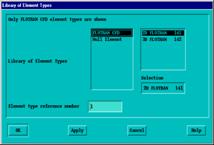
Define element type.
|
Add an element type. | |||
|
Choose 2D FLOTRAN element (FLUID141). OK. | |||
|
Close the Element Types Box. |
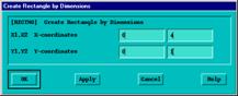
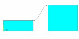
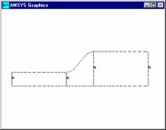
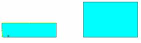
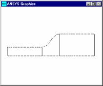
Create rectangle for the inlet region.
|
Enter X1=0, X2=4. Enter Y1=0, Y2=1. | |||
|
|
|||
Create the outlet rectangle.
|
Enter Y1=0, Y2=2.5. OK. | |||
|
Toolbar: SAVE_DB |
|||
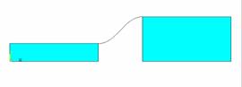
Create the transition region between the rectangles.
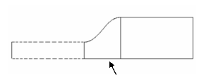
The transition region, where the flow expands, is bordered on the top by a smooth line tangent to the upper line of both rectangles. This line is created with the "Tangent to 2 lines" option. Note that the prompt in the Input Window will indicate what is to be picked (lines, ends of lines).
The area is then created as an arbitrary area through the four keypoints. Note that the area will be bounded by existing lines through those keypoints.
Main Menu: Preprocessor
-Modeling-Create
-Lines-Lines
Tan
to 2 Lines.
![]()
![]()
Pick the first line (upper line of left rectangle).
OK (in picking menu).
Pick the tangency end of the first line (upper right corner).
OK (in picking menu).
Pick the second line (upper line of the larger rectangle).
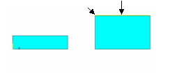
OK (in picking menu).
Pick the tangency end of the second line.
OK to create the line.
The result is a smooth line between the two areas.
Now create the third area as an arbitrary area through keypoints.
|
Pick 4 corners in counterclockwise order. OK. Toolbar: SAVE_DB. |
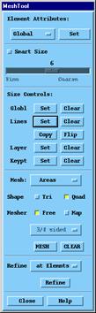
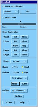
Establish mesh patterns
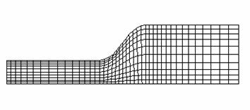
To create a mapped mesh, set the specific size controls along the lines (LESIZE command). The establishment of a good finite element mesh is quite important in CFD analyses.
The general finite element philosophy of putting more elements in regions with higher solution gradients applies here. The mesh density should be sufficient to enable the program to capture the nature of the phenomena. For example, a small recirculation region is likely to develop in the expansion region. The greater the number of applied elements implies a higher level of flow details that will be captured.
Apply 10 elements in the transverse direction (Y) and bias
them slightly towards the top and bottom boundaries. This will help capture
boundary layer effects. For high Reynolds number problems, finer meshes should
be used. Along the inlet flow direction (X) in the inlet, use the number of
divisions tabulated below.
|
Mesh Division Strategy |
|
|
Transverse (Y) direction |
10 divisions - bias toward walls |
|
Inlet region, |
15 divisions - bias toward inlet and transition |
|
Transition region |
12 divisions - uniform spacing |
|
Outlet region (initial) |
15 divisions - larger elements near outlet |
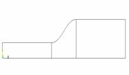
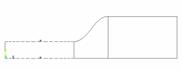
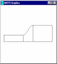
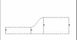
Before attempting this step, plot the lines for clarity.
|
| |||||
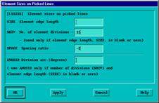
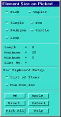
|
Choose Lines Set. Pick lines in flow direction along the inlet. |
|
Enter -2 as the Spacing ratio (this produces smaller elements near both ends of the line). Apply. |
The mesh ratio chosen results in smaller elements near the inlet, where the flow is developing, and near the expansion, in which more elements will be placed because of the high solution gradients in that region. There should be a relatively smooth transition in element size from region to region throughout the entire problem domain.
This process of picking the lines and entering the number of divisions and the ratios is repeated, using the mesh division strategy above. Note that the mesh division ratio is applied to the direction of the lines, the larger elements being at the end of the line. Thus the use of a number less than 1 for the upper line of the outlet region and a number greater than 1 for the lower line. (The line directions follow a counterclockwise direction, according to how they were generated.)
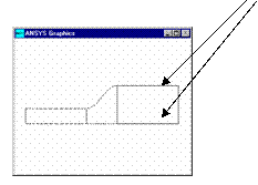
Transition region:
Pick
the top and bottom lines in the center area. ![]()
![]()
Apply (leaves the Picker Open to do the next set of lines).
Enter 12 as the No. of element divisions.

Enter 1 as the Spacing ratio (uniform spacing).
Apply.
Outlet region:
Pick the top and bottom lines in the outlet region.
Apply.
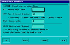
Enter 15 as the No. of element divisions.
Enter 3.0 as the Spacing ratio (bias towards outlet).
OK.
Notice that the upper line is not biased towards the outlet. The line bias needs to be "flipped."
 Choose Flip in the Mesh Tool.
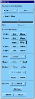

Pick the upper line only.
OK.
|
Choose Lines Set. Picker arises. Pick the 4 transverse direction lines. OK to close picking menu. | |||||
|
Enter -2 as the Spacing ratio (bias towards top and bottom walls). OK. Toolbar: SAVE_DB |
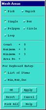
Create the finite element mesh.
|
Choose Mesh. Pick All. Close the Mesh Tool. |
|